Life-Cycle Benefit-Cost Analysis of Safety Related Improvements on Roadways

Transcription

1 Brigham Young University BYU ScholarsArchive All Theses and Dissertations Life-Cycle Benefit-Cost Analysis of Safety Related Improvements on Roadways Jordan Browne Frustaci Brigham Young University Follow this and additional works at: Part of the Civil and Environmental Engineering Commons BYU ScholarsArchive Citation Frustaci, Jordan Browne, "Life-Cycle Benefit-Cost Analysis of Safety Related Improvements on Roadways" (2016). All Theses and Dissertations This Thesis is brought to you for free and open access by BYU ScholarsArchive. It has been accepted for inclusion in All Theses and Dissertations by an authorized administrator of BYU ScholarsArchive. For more information, please contact

2 Life-Cycle Benefit-Cost Analysis of Safety Related Improvements on Roadways Jordan Browne Frustaci A thesis submitted to the faculty of Brigham Young University in partial fulfillment of the requirements for the degree of Master of Science Mitsuru Saito, Chair Grant G. Schultz Daniel P. Ames Department of Civil and Environmental Engineering Brigham Young University Copyright 2016 Jordan Browne Frustaci All Rights Reserved

3 ABSTRACT Life-Cycle Benefit-Cost Analysis of Safety Related Improvements on Roadways Jordan Browne Frustaci Department of Civil and Environmental Engineering, BYU Master of Science The Highway Safety Manual (HSM) lists four different methods for determining the change in crash frequency in order of reliability. Currently, the Utah Department of Transportation (UDOT) uses the fourth reliable method. The goal of this research was to develop a tool that the most reliable method mentioned in the HSM could be used to perform life-cycle benefit-cost analyses. A spreadsheet program was built that performs the HSM s Part C Predictive Method for 11 different roadway segment types mentioned in HSM using Excel macros and Visual Basic for Applications (VBA) programming. Intersections were not included in this spreadsheet program as they were not included in the Utah Crash Prediction Model (UCPM) or the Utah Crash Severity Model (UCSM) at the time of this research. The methodology for analysis was set up to become part of the use of the models in selecting countermeasures. The concept and spreadsheet layout are discussed using the rural two-lane two-way (TLTW) highway spreadsheet as an example. Three examples are presented in this thesis, which are a case of rural TLTW highway, a case of five-lane urban arterial with a two-way left-turn lane (TWLTL), and a case of a freeway segment, each with two selected countermeasures to compare their benefit-cost ratios (BCRs). One important aspect associated with life-cycle benefit-cost analysis of safety related improvements is the cost of countermeasures. The spreadsheets developed in this research can predict the benefits associated with a countermeasure following the methods found in the HSM; however, it does not include a module to estimate costs associated with a countermeasure to be selected because costs of countermeasures are dependent on the way such improvements are included in construction contracts. The engineer should seek guidance from the cost estimate expert within the agency or outside consultants when determining the project costs. Keywords: life-cycle, benefit-cost, safety, analysis

4 ACKNOWLEDGEMENTS This research would not have been possible without the efforts of many people. I am grateful to the Utah Department of Transportation (UDOT) which provided the funding for this research. Also, I could not have completed this research were it not for the assistance and expertise of the technical advisory committee for this study, especially W. Scott Jones of UDOT Traffic and Safety and Dallas Wall of WCEC. I am also grateful to the faculty and students on the research team at Brigham Young University. Specifically, I would like to thank Dr. Mitsuru Saito, Dr. Grant G. Schultz, and Dr. Daniel P. Ames for their guidance and assistance with this research, in addition to their mentoring throughout my education. Also, I would like to thank Josh Gibbons, Samuel Mineer, and Natalia Brown who provided assistance with VBA programming. I would also like to acknowledge the continued support and encouragement from my family. They have always been there for me and have supported me in whatever I set out to do. I would like to especially thank my father Samuel Frustaci and my step-mother Toni Frustaci, as well as my mother Patricia Frustaci. They have been my rock and support through my entire academic endeavor and would not be where I am today without them.

5 TABLE OF CONTENTS LIST OF TABLES... vi LIST OF FIGURES... vii 1 Introduction... 1 Background... 1 Purpose and Need... 3 Organization Literature Review... 5 Traffic Safety Defined... 5 UCPM... 7 SPFs... 9 CMFs Combining Multiple CMFs CMF Clearinghouse HSM Method HSM for Determining Change in Crash Frequency HSM Method for Converting Change in Crash Frequency to Monetary Benefit HSM Method for Determining Project Costs Economic Evaluation Method for Individual Sites Non-Monetary Considerations UDOT Method Chapter Summary Methodology Part C Predictive Method Life-Cycle Benefit-Cost Analysis Fundamentals Chapter Summary Concept And Spreadsheet Development Layout of Spreadsheet Program Basic Information Worksheet Analysis Worksheet Output Worksheets Spreadsheet Development in Excel Spreadsheet Analysis Procedure iv

6 Chapter Summary Application Through Example Rural TLTW Example Widening the Shoulder Adding a Passing Lane Five-Lane Arterial Including TWLTL Example Removing On-Street Parking Installation of Roadway Lighting Freeway Segment Example Installation of Inside and Outside Shoulder Rumble Strips Implementation of Automated Speed Enforcement Project Costs Chapter Summary Conclusions and Recommendations Conclusions Issues Related to Life-Cycle Benefit-Cost Analysis Difficulty with Using the EB Method in the Life-Cycle Benefit-Cost Analysis Difficulty with Crash Severity Distributions Limitations of Spreadsheet Program Recommendations References List Of Acronyms Appendix A. HSM Chapter 10 CMFs Appendix B. Application Through Example Supplements Appendix C. Software Availability v

7 LIST OF TABLES Table 2-1: Example of Service Life for Different Countermeasures from Various States Table 2-2: Crash Cost Summary Table Table 2-3: Benefit Value Per Crash Provided by the FHWA for Each Crash Type Table 2-4: Benefit Value Per Crash Provided by UDOT for Each Crash Type vi

8 LIST OF FIGURES Figure 2-1: UDOT Safety Programs Benefit/Cost Worksheet Crash Data Entry Figure 2-2: UDOT Safety Programs Benefit/Cost Worksheet CMF and Crash Reduction Figure 2-3: UDOT Safety Programs Benefit/Cost Worksheet BCR Figure 4-1: Basic Information Worksheet Example Figure 4-2: Inputs of Example Analysis Worksheet Figure 4-3: CMF Portion of Example Analysis Worksheet Figure 4-4: Observed Crash Frequency of Example Analysis Worksheet Figure 4-5: Crash Distribution of Example Analysis Worksheet Figure 4-6: SPF Information of Example Analysis Worksheet Figure 4-7: Crash Benefits and Costs of Example Analysis Worksheet Figure 4-8: Improvement Costs of Example Analysis Worksheet Figure 4-9: BCR of Example Analysis Worksheet Figure 4-10: VBA Buttons Used to Perform Analysis and Print Reports Figure 4-11: Example Analysis Worksheet Figure 4-12: Basic Output Figure 4-13: CMF and SPF Reports Figure 4-14: Benefit Table Figure 4-15: Cost Table Figure 4-16: Basic Information Worksheet for Example Analysis Figure 4-17: Roadway Characteristics for Example Analysis Figure 4-18: CMFs for Example Analysis Figure 4-19: Observed Crash Frequency for Example Analysis Figure 4-20: Crash Severity Distribution for Example Analysis Figure 4-21: SPF Results for Example Analysis Figure 4-22: Benefit Table Results for Example Analysis Figure 4-23: Benefit Results for Example Analysis Figure 4-24: Inputs for Cost Analysis Figure 4-25: Cost Table Results for Example Analysis Figure 4-26: BCR for Example Analysis vii

9 Figure 5-1: Basic Info Rural TLTW Example Figure 5-2: Roadway Segment Characteristics for Rural TLTW Example Figure 5-3: CMFs for Rural TLTW Example Figure 5-4: Observed Crash Frequency for Rural TLTW Example Figure 5-5: Crash Distribution for Rural TLTW Example Figure 5-6: SPF Results for Rural TLTW Example Figure 5-7: Total Benefits for Rural TLTW Example Figure 5-8: Costs for Rural TLTW Example Figure 5-9: Cost-Benefit Results for Rural TLTW Example Figure 5-10: Complete Spreadsheet for Rural TLTW Example Figure 5-11: Roadway Segment Characteristics for Second Rural TLTW Example Figure 5-12: CMF for Second Rural TLTW Example Figure 5-13: SPF Results for Second Rural TLTW Example Figure 5-14: Total Benefits Results for Second Rural TLTW Example Figure 5-15: Total Cost Results for Second Rural TLTW Example Figure 5-16: BCR Results for Second Rural TLTW Example Figure 5-17: Complete Spreadsheet for Second Rural TLTW Example Figure 5-18: Basic Info for Urban/Suburban 5T Arterial Example Figure 5-19: Roadway Segment Characteristics for 5T First Example Figure 5-20: CMFs for 5T First Example Figure 5-21: Observed Crash Frequency and Crash Distribution for 5T First Example Figure 5-22: SPF Results for First 5T Example Analysis Figure 5-23: Total Benefits for First 5T Example Figure 5-24: Total Costs for First 5T Example Figure 5-25: BCR for First 5T Example Figure 5-26: Entire 5T Spreadsheet for First 5T Example Figure 5-27: Roadway Segment Characteristics for Second 5T Example Figure 5-28: CMFs for Second 5T Example Analysis Figure 5-29: SPF Results for Second 5T Example Figure 5-30: Total Benefits for Second 5T Example Figure 5-31: Total Costs for Second 5T Example viii

10 Figure 5-32: BCR for Second 5T Example Figure 5-33: Entire Spreadsheet for Second 5T Example Figure 5-34: Basic Info for Freeway Segment Example Figure 5-35: Roadway Segment Characteristics for First Freeway Segment Example Figure 5-36: CMFs for First Freeway Segment Example Figure 5-37: Observed Crash Frequency and Crash Distribution for Freeway Examples Figure 5-38: SPF Results for First Freeway Segment Example Figure 5-39: Total Benefits for First Freeway Segment Example Figure 5-40: Total Costs for First Freeway Segment Example Figure 5-41: BCR for First Freeway Segment Example Figure 5-42: Entire Spreadsheet for First Freeway Segment Example Figure 5-43: Roadway Segment Characteristics for Second Freeway Example Figure 5-44: CMFs for Second Freeway Example Figure 5-45: SPF Results for Second Freeway Segment Example Figure 5-46: Total Benefits for Second Freeway Segment Example Figure 5-47: Total Costs for Second Freeway Segment Example Figure 5-48: BCR for Second Freeway Segment Example Figure 5-49: Entire Spreadsheet for Second Freeway Segment Example ix

11 1 INTRODUCTION Safety on roadways is one aspect under consideration when roadways are being rebuilt, rehabilitated, or maintained. One important aspect when considering safety are life-cycle benefitcost analyses. Life-cycle benefit-cost analysis is one necessary step to be performed with different safety countermeasures to determine which safety countermeasure provides the best benefit for the lowest cost. This research explores how these analyses can be performed using spreadsheets. This chapter presents the background information related to this research, explains the purpose and need for this research, and the organization of the report. Background Safety on roadways is important everywhere. The Utah Department of Transportation (UDOT) has made it one of its top priorities, which can be seen in their campaign: Zero Fatalities: A Goal We Can All Live With TM. This campaign is all about eliminating fatalities on [Utah] roadways (Zero Fatalities 2016). One way that UDOT accomplishes this goal of Zero Fatalities is by performing safety related improvements on roadway segments that have experienced a greater number of crashes than expected. When determining which safety related improvement will be most effective, various analyses must be performed. One of these analyses is a life-cycle benefit-cost analysis. 1

12 The Highway Safety Manual (HSM) presents the preferred methods for performing lifecycle cost benefit analyses of safety related improvements (AASHTO 2010a). Part of the lifecycle benefit-cost analysis of safety related improvements is to determine the change in the number of expected crashes for each proposed improvement. The HSM contains a process for determining the change in average crash frequency known as the Part C Predictive Method. The Part C Predictive Method is an 18-step method for predicting average crash frequencies. The Part C Predictive Method includes numerous predictive models that use safety performance functions (SPFs), crash modification factors (CMFs), and other factors to predict the number of crashes that a roadway segment or intersection will experience based on its physical characteristics. SPFs are regression models that estimate the average crash frequency for a specific roadway type as a function of the annual average daily traffic (AADT), segment length, and regression constants. These constants are determined based on the crash severity being considered and the roadway type. A CMF is an index of how much a crash rate is expected to change following a physical change in the roadway or intersection. A CMF is simply a ratio between the number of crashes per unit of time expected after a modification or an improvement measure is implemented and the number of crashes per unit of time estimated if the change does not take place (AASHTO 2010a). The HSM outlines four different methods for determining the change in crashes in order of reliability. The most reliable method is the Part C Predictive Method, while the least reliable method uses observed crash data and applies a CMF without considering SPFs. Currently UDOT uses the latter method to determine the change in average crash frequency when performing benefit-cost analyses of safety related improvements. This research is intended to create a 2

13 method in which UDOT can use the Part C Predictive Method as part of the life-cycle benefitcost analyses of safety related improvements. Purpose and Need The purpose of this research is to develop an Excel-based spreadsheet program that performs life-cycle benefit-cost analysis for safety related improvements using the method ranked most reliable in the HSM. This Excel-based spreadsheet program uses the Part C Predictive Method to determine the reduction in crash frequency, and uses the life-cycle, present value analysis method presented in Volume 1 of the HSM (AASHTO 2010a). The Part C Predictive Method does not have information for every type of roadway. The scope of this research includes 11 roadway types included in the HSM (AASHTO 2010a): 1. Rural two-lane two-way (TLTW) highways 2. Undivided rural multilane highways 3. Divided rural multilane highways 4. Two-lane undivided suburban/urban arterials 5. Three-lane suburban/urban arterials including a two-way left-turn lane (TWLTL) 6. Four-lane undivided suburban/urban arterials 7. Four-lane divided suburban/urban arterials 8. Five-lane suburban/urban arterials including a TWLTL 9. Rural and urban freeway segments 10. Freeway speed change lanes 11. Freeway ramps The need for this research arose as UDOT does not currently use the most reliable method for performing life-cycle benefit-cost analyses of safety related improvements. The 3

14 purpose of life-cycle benefit-cost analyses is to help the safety engineer to determine which improvement will create the largest safety benefit compared to its cost. These analyses are essential because they are used to determine which improvements should be chosen and how tax payer money is used to benefit the public. Hence, it is important to perform the most accurate analysis possible recommended by the HSM to make sure that money is used effectively and to achieve the highest possible reduction of crashes. As part of a previous and current research effort by Brigham Young University (BYU), the Utah Crash Prediction Model (UCPM) and Utah Crash Severity Model (UCSM) were developed (Schultz et al. 2015). These models are only used for roadway segments and cannot be used for intersections and interchanges at the time of this research. Since this research effort was in conjunction with the research effort for these models, intersections and interchanges were not included as part of the spreadsheets for this life-cycle benefit-cost analysis of safety related improvements. Organization This thesis consists of seven chapters. Chapter 1 presented an overview of the report along with a stated purpose and need for this research. Chapter 2 contains the literature review, which is a summary of topics related to the research. Chapter 3 explains the methodology used in this research project. Chapter 4 discusses the concept used in this research including the software development. Chapter 5 includes three sample applications: a rural highway, a suburban/urban arterial, and a freeway. Chapter 6 contains a discussion about the findings of the research. Chapter 7 contains conclusions and recommendations for use of the Excel-based spreadsheet program as well as possible further research projects. Following the body of the report, there are appendices that include sources and information that were used to complete this research. 4

15 2 LITERATURE REVIEW A literature review was performed on traffic safety and the life-cycle benefit-cost analysis of safety related improvements. This chapter presents a background into traffic safety, the UCPM, SPF, CMF, the HSM method for performing life-cycle benefit-cost analysis of safety related improvements, and the current UDOT method for performing life-cycle benefit-cost analysis of safety related improvements. For more detail on the safety and crash analysis techniques, the reader should refer to previous research related to this topic conducted by BYU researchers (Saito et al. 2010, Schultz et al. 2011, Schultz et al. 2012, Schultz et al. 2013, Schultz et al. 2014, Schultz et al. 2015). Traffic Safety Defined The HSM defines safety as the crash frequency or crash severity, or both, and collision type for a specific time period, a given location, and a given set of geometric and operational conditions (AASHTO 2010a). There are two categories for safety: subjective and objective. Subjective safety concerns the perception of how safe a person feels on the transportation system. Objective safety is the use of a quantitative measure that is independent of the observer. Regardless of which type of safety metric is used, the general consensus is that the number of crashes on a roadway can help determine the level of safety on the roadway. The HSM defines a crash as a set of events that result in injury or property damage due to the collision of at least 5

16 one motorized vehicle and may involve collision with another motorized vehicle, bicyclist, pedestrian, or object (AASHTO 2010a). Crash frequency is defined as the number of crashes occurring at a particular site, facility, or network in a one-year period (AASHTO 2010a). There are many factors that affect the number of crashes that occur on a roadway such as speed, roadway design, roadside design, median treatments, auxiliary lanes, horizontal and vertical alignment, lane and shoulder widths, shoulder types, and other cross-sectional elements (AASHTO 2011). Based on these definitions and the idea that safety is based on crashes and crash frequency, the higher the crash frequency, the less safe a roadway segment is perceived to be. Safety has continued to become a focus for transportation officials and continues to be a critical aspect in the transportation decision making process (Tobias 2016). This thesis will help illustrate how safety can be integrated into the transportation decision making process. Another major part of safety is crash severity. The HSM uses the KABCO scale, which separates different crashes into various categories based on how severe the crashes are. The different categories are outlined as follows (AASHTO 2010a). K Fatal injury A Incapacitating injury B Non-incapacitating injury C Possible injury O No injury/property Damage Only (PDO) Crash severity can be helpful in determining which roadway segments truly are the least safe, as there may be segments with a high number of crashes, but all of them a type C or O while other segments may have a low number of crashes, but most of them are type K, A, and B 6

17 crashes. While UDOT definitely does not want crashes of any kind, their focus is on fatal injury crashes, which means that they would probably prefer to focus on segments that had a high number of fatal injury crashes, even if the overall number of crashes was lower when compared to other segments. Safety has been a focus at UDOT for quite a while. To help with reducing the number of fatal injury crashes and crashes in general in Utah, two models have been created in previous research projects: UCPM and UCSM. The UCPM is used to predict the total crash frequency including all types of crashes that will take place on a given roadway segment, while the UCSM is used to determine which roadway segments have the highest number of severe injury crashes (Schultz et al. 2015). Since this research is focused on the life-cycle benefit-cost exploration, the UCPM will be more useful than the UCSM. The UCPM will be explained in further detail in the following section. UCPM In previous research efforts by BYU, the UCPM was developed to help UDOT identify sections that could have a higher number crashes than expected (Schultz et al. 2015). In this model, a variety of parameters such as vehicle-miles traveled (VMT), number of lanes, speed limit, and others are used to create a crash distribution for different road segments. The mean of the distribution is used as the expected number of crashes that might occur on a specific segment based on the characteristics of that segment (Saito et al. 2011). In this model, a pre-selection process is performed using the Bayesian horseshoe selection method, which takes all possible parameters in the dataset and produces a list of the significant ones that should be used. The selected parameter set can be used to predict the number of crashes for a given severity group. 7

18 To start the procedure, a statistical model must be chosen to provide the base dataset in the analysis and identification of the problem segments or hot spots. The analysis that was completed in the previous research project used a statistical model that included all of the crashes from the years 2008 to 2012 (Schultz et al. 2015). The data for the model used included the total crash counts for each segment and the count of crashes for each attribute selected by the Bayesian horseshoe selection method. The UCPM required 100,000 iterations to obtain posterior predictive distributions on the number of crashes expected to occur on each segment. This model included total crash counts for both all severity levels and the severity level A and K. The UCPM compared the actual number of crashes to the posterior predictive distribution of crash occurrences to determine the percentile for each segment as a number between 0 and 1. This percentile was used to rank each of the segments. The higher the percentile the higher the ranking for the segment. Along with other outputs of the model, the data entered into the model were used to determine the probability that the expected number of crashes actually occurred. This probability was also used in the ranking process. As this model can be used to determine the number of crashes that are expected to occur on a given roadway segment, it can help determine the number of crashes that will be reduced on each roadway segment when the values of the selected variables are changed. As this model can also be used to determine number of each severity type crash, this can be useful in determining how many of each severity type will be reduced on a given roadway segment. The UCPM combined with SPFs and CMFs can help to obtain a reliable estimate of the number of crashes that can be reduced on a roadway segment. After the number of crashes reduced is determined, the benefit can be determined by comparing different possible treatments to improve safety. The 8

19 following sections further explore SPFs and CMFs and how they can work in determining the change in crash frequency on a roadway segment. SPFs SPFs are regression models that estimate average crash frequency for a specific site type as a function of AADT and segment length. There are base conditions such as lane width, lighting characteristics, turn lanes, and others that can be specified for each SPF (AASHTO 2010a). Equation 2-1 provides an example of a SPF for rural TLTW highways from the HSM (AASHTO 2010a) (2-1) where, Nspf = number of predicted annual crashes, AADT = average annual daily traffic (vehicles per day), and L = segment length (mi). This SPF converts AADT into VMT per year by multiplying AADT by the segment length (L). By multiplying VMT by 10-6, the model converts predicted number of crashes into million VMT per year, which makes the number of predicted annual crashes much easier to work with. The constant e or exponential is used in calculating the appropriate regression factors. The HSM contains SPFs for three facility types (rural TLTW roads, rural multilane highways, and urban and suburban arterials). There are also SPFs for specific site types of each facility (signalized intersections, un-signalized intersections, divided roadway segments, undivided roadway segments). In order to apply an SPF, there are three pieces of information that must be known for the study site. The basic information of the study site is used to 9

20 determine whether an SPF is available for that facility and site type. The detailed geometric design and traffic control features of the site are then required to determine whether the conditions of the study site vary from the SPF baseline conditions. The AADT and traffic growth rate must also be known to help forecast estimates of AADT for future periods (AASHTO 2010a). The SPFs in the HSM are developed using observed crash data collected over a number of years, but with the data from limited number of states and calibration is needed to reflect local conditions. The parameters of the SPFs are determined by assuming that the crash frequencies follow a negative binomial distribution. The negative binomial distribution is better suited for the crash data as opposed to the often-used Poisson distribution because the Poisson distribution is generally used when the mean and the variance of the data are equal. In the case of crash data, the variance usually exceeds the mean, which is defined as over-dispersed. The amount of over-dispersion is represented by a statistic, known as the over-dispersion parameter, which is one of the statistics provided by statistical software programs. The larger the dispersion parameter, the more the crash data vary as compared to a Poisson distribution with the same mean and variance (AASHTO 2010a). SPFs tend to be simplistic and have certain limitations as they estimate crash frequency for all crashes and do not separate the estimated crash frequency into components by crash severity levels and collision types (such as run-off-the-road or rear-end crashes). SPFs use a variety of different parameters such as speed limit, lane width, shoulder width, etc. and any number of parameters can be used in the model. The goal is to choose the correct parameters for the roadway segment under consideration. The SPF should be calibrated using local conditions to make the model applicable to the given segment. The SPFs in the HSM are based off of general 10

21 conditions such as 12-foot lane widths, six-foot paved shoulders, etc. If the segments that are being examined differ from these conditions, then the model should be adjusted to the local conditions by changing the parameters in the SPF or by using CMFs. Another limitation of SPFs is that they contain predictive factors as opposed to causal factors such as human factors since human factors are difficult to model and reflect in mathematical models. Since there are these limitations to SPFs, the SPFs need to be adjusted, which is done by using CMFs (AASHTO 2010b). CMFs are discussed in section 2.4. CMFs The HSM defines CMFs as the relative change in crash frequency due to a change in one specific condition, estimating the effect of a particular geometric design or traffic control or the effectiveness of a particular treatment or condition (AASHTO 2010a). CMFs were originally referred to as Accident Modification Factors (AMFs), but were changed in the final version of the HSM to be CMFs (Fitzpatrick et al. 2008). CMFs can be used to determine the effectiveness of a particular treatment or condition. CMFs are usually presented for the implementation of a particular treatment, which is also known as a countermeasure, intervention, action, or alternative design (Gross et al. 2010). Most CMFs have to do with roadway characteristics such as the shoulder width, lane width, presence of rumble strips, etc. (AASHTO 2010a). CMFs are the ratio of the crash frequency of a site under two different conditions. Generally, the ratio is the number of crashes after a particular roadway change divided by the number of crashes before the change took place. If a CMF is equal to 1.00, this means that there was no change in the number of crashes on a roadway segment. If the CMF is greater than 1.00, the number of crashes has increased, and if the CMF is less than 1.00 the number of crashes has 11

22 decreased. The CMF can also be used to calculate the percent in crash reduction. The equation for the percent in crash reduction is shown in Equation 2-2. Percent Reduction in Crash=100 ( CMF) (2-2) Essentially, CMFs are the percent of crashes that occurred after the change, while the percent reduction in crashes is the percent of crashes that were removed or increased after the change. For example, if the CMF is 0.6, then the percent reduction in crashes is 40% (100x(1-0.6)). This means that after the change only 60% of the crashes occurred and there was a 40% reduction. If the CMF is 1.3, then the percent reduction in crashes is -30% or a 30% increase in crashes. The HSM presents CMF values in three different formats. The CMFs are presented either in text, in a formula referred to as a Crash Modification Function, or in a tabular form. Text is usually used when there is a limited range of options for a particular treatment; a formula is used where treatment options are continuous variables; tabular form is used where the values vary by facility type. When CMFs are determined using an equation or graph, or when the CMF is presented as a discrete value, the CMF is typically rounded to two decimal places (AASHTO 2010a). The following subsections will give more pertinent information regarding CMFs Combining Multiple CMFs Many times when roadway improvements or treatments take place, there are multiple treatments that are performed simultaneously. This creates a compound effect on crash reduction. The general practice is to multiply all of the CMFs together to produce a new CMF. For example, if a given roadway segment was to have two treatments, one with a CMF of 1.2 and the 12

23 other with a CMF of 0.5. The overall CMF for the combination of treatments is 0.6 (1.2 x 0.5). There are cases where the treatments are not always compatible. Engineering judgment must be used when combining CMFs where multiple treatments change the overall nature of the site, and that different CMFs are not compatible. An example may be the installation of a roundabout at an urban two-way stop-controlled or signalized intersection. The usual procedure would be to try to estimate the current crash frequency and then apply a CMF for a conventional intersection to roundabout conversion. By installing the roundabout, the nature of the site is changed significantly and CMFs applicable to existing urban two-way stop-controlled or signalized intersections may no longer be relevant (AASHTO 2010a) CMF Clearinghouse The CMF Clearinghouse houses a web-based database of CMFs along with supporting documentation to help transportation engineers identify the most appropriate countermeasures for their safety needs. The CMF Clearinghouse also contains a great deal of resources to help in using the CMFs and SPFs. It also provides information on how to calibrate and use CMFs and SPFs (CMF Clearinghouse 2015). There is a section in the CMF Clearinghouse that also includes all of the information about CMFs such as a frequently asked questions section, a glossary to define useful terms regarding CMFs, the relationship of CMFs to the HSM, and the option to submit a CMF research need. There is also a User Guide on the CMF Clearinghouse that can be used to help users know how to use the CMF Clearinghouse website effectively. The user guide provides an introduction to CMFs in general as well as the CMF Clearinghouse. The CMF Clearinghouse also has a majority of the CMFs that can be used for different projects, and the user guide has instructions on how appropriate CMFs can be selected for specific projects. 13

24 There is also a section in the CMF Clearinghouse where a user can submit a CMF based on their personal research. The CMF Clearinghouse also has a section where it has a variety of resources that can be helpful for users. Some of these resources include resources for how to develop and use CMFs and how to develop and use SPFs. Trainings are also available on the CMF Clearinghouse to help train users when using CMFs and the HSM. The following items are also included in the CMF Clearinghouse: a section that explains how CMFs are used in conjunction with the HSM, numerous resources for countermeasure selection and for behavioral countermeasures, international resources with links to road safety for different countries around the world, numerous publications regarding CMFs and different updates on how CMFs have changed over time, and contact information for users to contact the pertinent person from the Federal Highway Administration (FHWA) Office of Safety Programs. Another useful feature of the CMF Clearinghouse is the information on life-cycle benefitcost analysis. The CMF Clearinghouse contains various spreadsheets that represent compilations of information useful in analysis. One valuable resource is a spreadsheet that is the compilation of information from all 50 states on the different lengths of service life that each state uses in determining how long each feature such as pavement, striping, or signing will last. An example of this spreadsheet can be seen in Table 2-1 (CMF Clearinghouse 2015). Table 2-1 shows a portion of the spreadsheet for four states: Alaska (AK) in 2014, Arizona (AZ) in 2010, California (CA) in 2013, and Connecticut (CT) in The complete version of this spreadsheet can be found on the CMF Clearinghouse and contains information for all 50 states. 14

25 Table 2-1: Example of Service Life for Different Countermeasures from Various States (CMF Clearinghouse 2015) AK AZ CA CT Alaska Highway Safety Improvement Program Handbook The Arizona Highway Safety Improvement Program Handbook Local Road Safety - A Manual for California's Local Road Owners Countermeasure Name Convert from two way traffic to one way traffic 20 Convert to one way frontage roads Convert two lane facility to four lane divided Improve drainage Increase turning radius Install acceleration/deceleration lane(s) 20 Install centerline rumble stripes Install centerline rumble strips 10 Install centerline rumble strips/stripes 10 Install climbing lane 20 Install edgeline rumble strips Install edgeline rumble strips/stripes 10 Install glare shields Install lane(s) 20 Install left turn acceleration lane Install one way couple Install passing lane(s) Install right turn acceleration lane Install rumble strips 10 Install rumble strips on approaches to intersections Install through lane(s) Install truck escape ramp 20 Install turnabout Another valuable resource in the CMF Clearinghouse is the crash cost summary table, which includes all of the values for each state of how much they value the cost of each crash. For example, a fatal injury crash has a much higher cost than a non-injury crash. A portion of the crash cost summary table can be seen in Table 2-2. These resources can be helpful in determining the life-cycle benefit-cost analysis of a roadway improvement or change. 15

26 Table 2-2: Crash Cost Summary Table (CMF Clearinghouse 2015) Cost of Incapacitating Injury Crash (A) Cost of Non- Incapacitating Injury Crash (B) Cost of Property Damage Only Crash (O) State Cost of Fatal Crash (K) Cost of Possible Injury Crash ( C ) AK AZ CA CO DE IA Actual value ID IL IN KS KY HSM Method The HSM can be considered the basis for anything related to safety on roadways. This also applies to life-cycle benefit-cost analysis of safety related improvements and the method explained in the HSM can be considered the preferred method to complete this type of analysis. The specific details associated with the HSM Method can be found in the following subsections HSM for Determining Change in Crash Frequency The benefits of safety for a project are determined using the crash information for a site. One of the most important parts of completing a life-cycle benefit-cost analysis of safety related improvements is to estimate the change in the number of crashes for a proposed project. The HSM outlines four different methods for estimating the change in expected average crash frequency of a proposed project or project design alternative (AASHTO 2010a). The Part C Predictive Method has a part in each of the four methods. The Part C Predictive Method refers to the method outlined in Volume 2 of the HSM (AASHTO 2010b). This method provides procedures to estimate the expected average crash frequency when geometric design and traffic 16

27 control features are specified (AASHTO 2010b). When the Part C Predictive Method is not available to be used, the Part D of the HSM method can be used instead. Part D presents a number of CMFs to represent how a certain modification will affect the crash frequency of a given roadway segment (AASHTO 2010b). The four methods listed in the Part C are presented below in order of reliability: Method 1 Apply the Part C Predictive Method to estimate the expected average crash frequency of both the existing and proposed conditions Method 2 Apply the Part C Predictive Method to estimate the expected average crash frequency of the existing condition, and apply an appropriate project CMF from Part D to estimate the safety performance of the proposed condition. Method 3 - If the Part C Predictive Method is not available, but an SPF applicable to the existing roadway condition is available (i.e., an SPF developed for a facility type that is not included in Part C), use that SPF to estimate the expected average crash frequency of the existing condition, and apply an appropriate project CMF from Part D to estimate the expected average crash frequency of the proposed condition. A locally derived project CMF can also be used in Method 3. Method 4 Use observed crash frequency to estimate the expected average crash frequency of the existing condition, and apply an appropriate project CMF from Part D to the estimated expected average crash frequency of the existing condition to obtain the estimated expected average crash frequency for the proposed condition. This method is applied to facility types not addressed by the Part C Predictive Method. 17

28 When a CMF from Part D of the HSM is used in one of the four methods, the associated standard error of the CMF can be applied to develop a confidence interval around the expected average crash frequency estimate. This range can help the analyst to see what type of variation could be expected when implementing a countermeasure. When there is no applicable Part C Predictive Method, SPF, and CMF, the HSM procedures cannot provide an estimate of the expected project effectiveness. In order to evaluate countermeasures, engineering judgment may be used to develop an estimated applicable CMF. The results of the analysis would be considered uncertain, and a sensitivity analysis based on a range of CMF estimates could be used to support decision-making (AASHTO 2010a) HSM Method for Converting Change in Crash Frequency to Monetary Benefit After the change in crashes has been estimated for a project, the benefits from preventing the crashes needs to be converted into a monetary value. The first step in converting the benefits to a monetary value is to calculate the annual monetary value. To calculate the annual monetary value for the benefits of reducing crashes, multiple data are needed. The accepted monetary value of crashes by severity is needed to determine how the reduction in each crash severity level has created a benefit for the project. There are numerous differing opinions on how these values of the different crash types should be calculated. The FHWA has completed a significant amount of research that establishes a basis for quantifying, in monetary terms, the human capital crash costs to society of fatalities and injuries from highway crashes. These estimates include the monetary losses associated with medical care, emergency services, property damage, lost productivity, etc. to society as a whole. The FHWA values for each crash severity level can be seen in Table 2-3 (AASHTO 2010a). 18

29 Table 2-3: Benefit Value Per Crash Provided by the FHWA for Each Crash Type (AASHTO 2010a) Severity Severity Severity No. Value PDO O 1 7, Possible Injury C 2 44, Evident Injury B 3 79, Disabling Injury A 4 216, Fatal K 5 4,008, State and local jurisdictions often have accepted societal crash costs by crash severity and collision type. For example, UDOT has their own monetary values that they use in determining the value of each crash severity level (Wall 2016). There are five crash severity levels considered that are presented on a KABCO scale. As would be expected, fatal crashes have a higher value than PDO crashes. UDOT equalizes the scale for the fatal and disabling injuries so that the fatal crashes and the disabling injury crashes have the same monetary value. The values used by UDOT for each crash severity levels can be seen in Table 2-4 (Wall 2016). This is done to lessen the benefit provided by reducing fatal crashes and increase the benefit provided by reducing disabling injury crashes. While of course, fatal crashes are the crashes that should most definitely be prevented, in many cases, disabling injuries may cost more than fatal crashes in a long run because of lingering medical costs and the persons involved in these incapacitating injuries being prevented from ever working again. Other than these monetary values of crashes by severity, the change in crash estimates for different categories are also needed. 19

30 Table 2-4: Benefit Value Per Crash Provided by UDOT for Each Crash Type (Wall 2016) Severity Severity Severity No. Value PDO O 1 3, Possible Injury C 2 62, Evident Injury B 3 122, Disabling Injury A 4 Fatal K 5 1,961, ,961, After the change in crash benefit is converted into an annual value, the annual value must be converted into the present value. There are two different methods for converting the annual monetary benefits to present value. One method is where the annual benefits are uniform over the service life of the project, while the other method is where the annual benefits vary over the life of the project. The first method is used when the annual benefits are uniform over the service life of the project. In the first method, annual monetary benefits is multiplied by a conversion factor for a series of uniform annual amounts to present value to produce the present value of the project benefits for a specific site. The conversion factor is calculated using an equation that includes a minimum attractive rate of return or discount rate and the particular year in the service life of the countermeasure is being analyzed. This can be seen in Equation 2-3 (AASHTO 2010a).,,... (2-3) where, PA,i,y = Conversion factor for a series of uniform annual amounts to present value i = Minimum attractive rate of return or discount rate y = Year in the service life of the countermeasure(s) 20

31 The second method for converting the annual values to present values is used when the annual benefits vary over the service life of the project. Some countermeasures produce larger changes in expected crash frequency in the first years after the implementation than in subsequent years. In order to account for this occurrence over the service life of the countermeasure, non-uniform annual monetary values can be calculated as done in the first method. The first step in this method is to convert each annual monetary value to its individual present value. Each future annual value is treated as a single future value; therefore, a different present worth factor is applied to each year. The annual monetary benefits are multiplied by a different factor that converts a single future value to its present value. The equation for the factor can be seen in Equation 2-4 (AASHTO 2010a).,, 1.0 (2-4) where, PF,i,y = Factor that converts a single future value to its present value i = Minimum attractive rate of return or discount rate y = Year in the service life of the countermeasure(s) After these values are all calculated, the next step is to sum the individual present values to arrive at a single present value that represents the overall benefits of the project HSM Method for Determining Project Costs After the benefits of the project are calculated the costs of the projects need to be estimated. Determining the costs associated with implementing a countermeasure follows the same procedure as performing cost estimates for other construction projects. Similar to other 21

32 roadway construction projects, expected project costs are unique to each site and to each proposed countermeasures. The cost of implementing a countermeasure or set of countermeasures could include a variety of factors, such as right-of-way acquisition, construction material costs, grading and earthwork, utility relocation, environmental impacts, maintenance, and planning and engineering design work conducted prior to construction (AASHTO 2003). Project costs are expressed as present values for use in economic evaluation. Project construction or implementation costs are typically already present values, but any annual or future costs for maintenance and operation need to be converted to present values using the same relationships presented in section for project benefits (AASHTO 2010a) Economic Evaluation Method for Individual Sites After the benefits and costs are both calculated, the economic evaluation can be performed for the project sites. There are two steps in performing the economic evaluation: determine if a project is economically justified (the benefits are greater than the costs), and determine which project or alternative is most cost-effective. This section will explain different ways the most cost-effective improvement alternative can be determined. The first step is to determine if a project is economically justified is by using the Net Present Value (NPV) method, which is also referred to the Net Present Worth (NPW) method (AASHTO 2010a). This method is used to express the difference between the present cost and present benefit of an individual improvement project in a single amount. The NPV or NPW method can be used for two basic functions. This method can be used to determine which countermeasure or set of countermeasures provides the most cost-efficient means to reduce crashes. The countermeasures or sets of countermeasures are ordered from the highest to lowest NPV. The method can also be used to evaluate if an individual project is economically justified. 22

33 Its first step is to estimate the number of crashes reduced due to the safety improvement project. The crash reduction is then converted to an annual monetary benefit. This annual monetary benefit is then converted to a present value. The present value of the costs associated with implementing the project is then calculated. These benefits and costs are then entered into Equation 2-5 to determine the NPV. (2-5) where, NPV = Net present value of the project PVbenefits = Present value of the project benefits PVcosts = Present value of project costs A project with a NPV greater than zero indicates a project with benefits that are sufficient enough to justify implementation of the countermeasure. A value less than zero indicates a project that does not produce enough benefits to justify implementation of the countermeasure. There are strengths and weaknesses associated with the NPV analysis method. The strengths are that it evaluates the economic justification of a project, the NPV are ordered from highest to lowest, and it ranks the projects with the same rankings as produced by the incremental benefit-to-cost ratio method. One weakness of this method is that the magnitude cannot be easily interpreted as a benefit-cost ratio (BCR). This is because only the total monetary net benefit is calculated as opposed to comparing the benefits to costs. This method can help determine if a countermeasure is economically justified, but it does not necessarily determine which countermeasure would be the best. 23

34 After the NPV is calculated, a BCR can be calculated. A BCR is the ratio of the presentvalue benefits of a project to the implementation costs of the project. If the ratio is greater than 1.0, the project can be considered economically justified. After BCRs are calculated, countermeasures are then ranked from highest to lowest BCR. To calculate the BCR, the present value of the estimated change in average crash frequency and the present value of the costs associated with the safety improvement project need to be calculated. The BCR is calculated using Equation 2-6 (AASHTO 2010a). (2-6) where, BCR = Benefit-cost ratio PVbenefits = Present value of the project benefits PVcosts = Present value of project costs As stated previously, this method can only be used to determine the most valuable countermeasures for a specific site and can be used to evaluate economic justification of individual projects. Another procedure to produce a cost-effectiveness analysis is to not convert the predicted change in average crash frequency into monetary values, but to compare them directly to project costs. The cost-effectiveness of a countermeasure implementation project is expressed as the annual cost per crash reduced. Both the project cost and the estimated average crash frequency reduced must apply to the same time period, either on an annual basis or over the entire life of the project. This method requires an estimate of the change in crashes and cost estimate 24

35 associated with implementing the countermeasure. It is used to gain a quantifiable understanding of the value of implementing an individual countermeasure or multiple countermeasures at an individual site when an agency does not support the monetary crash cost values used to convert a project s change in estimated average crash frequency reduction to a monetary value. The first step in this cost-effectiveness analysis method is to estimate the change in expected average crash frequency due to the safety improvement project. The next step is to calculate the costs associated with implementing the project. The last step is to calculate the cost effectiveness of the safety improvement project at the site by dividing the present value of the costs by the estimated change in average crash frequency over the life of the countermeasure. This is shown in Equation 2-7. (2-7) where, PVcosts = Present value of project costs Npredicted = Predicted crash frequency for year y Nobserved = Observed crash frequency for year y The strengths associated with this method are that it results in a simple and quick calculation that provides a general sense of an individual project s value. It produces a numeric value that can be compared to other safety improvement projects evaluated with the same method, and there is no need to convert the change in expected average crash frequency by severity to a monetary value. The weakness is that it does not differentiate between the value of reducing a fatal crash, injury crash, and a PDO crash. 25

36 2.5.5 Non-Monetary Considerations While most cases will involve benefits being converted into monetary values and then comparing these values to the monetary costs, there are also cases where non-monetary considerations need to be taken into account. For example, many factors not directly related to changes in crash frequency enter into decisions about countermeasure implementation projects and many cannot be quantified in monetary terms. Examples of non-monetary considerations include: public demand, public perception and acceptance of safety improvement projects, meeting established and community-endorsed policies to improve mobility or accessibility along a corridor, road user needs, and others. For projects intended primarily to reduce crash frequency or severity, a benefit-cost analysis in monetary terms may serve as the primary decision-making tool, with secondary consideration of qualitative factors. The decision-making process on larger scale projects that do not focus only on change in crash frequency may be primarily qualitative or may be quantitative by applying weighting factors to specific decision criteria such as safety, traffic operations, air quality, noise, and others. While it is always easiest to determine the best alternative based on the monetary benefits, there are always other factors that should be taken into consideration (AASHTO 2010a). UDOT Method The current methods for performing a benefit-cost analysis at UDOT were explained to the BYU research team in an interview with Dallas Wall, an engineering consultant to UDOT. As explained in section 2.5.2, UDOT has a set of values that are used in calculating the monetary benefit for performing a specific type of crash. UDOT currently uses a model in which the CMF is multiplied by the number of crashes and then the reduction in crashes is determined. This reduction in the number of crashes is then used to calculate the monetary benefits based on the 26

37 crash costs explained previously. The benefits are then compared to the costs of implementing the possible countermeasure, which becomes the basis for benefit-cost analysis. The current UDOT model was found to follow the methods outlined in the HSM method summarized in section 2.5. The model has entries for crash data to be used as the existing average crash frequency. The crash data are generally observed crash data at the site from prior years. The place where the existing crash data can be entered can be seen in Figure 2-1 (Wall 2016). Figure 2-1: UDOT Safety Programs Benefit/Cost Worksheet Crash Data Entry (Wall 2016) There are also entries for the various CMFs that are applicable to the various countermeasures. The current UDOT model allows for the use of various countermeasures. The model allows the user to enter the number of crashes that will be affected by each 27

38 countermeasure. These crashes are then multiplied by their respective CMFs to determine the reduction in crashes. This part of the spreadsheet can be seen in Figure 2-2. Figure 2-2: UDOT Safety Programs Benefit/Cost Worksheet CMF and Crash Reduction (Wall 2016) The reductions in crash frequency calculated using the UDOT model are then converted into annual monetary values by multiplying the reduced number of each crash type by the corresponding monetary benefit for each crash and then multiplying these monetary benefits by a conversion factor. The conversion factor used in this model is the conversion factor for a series of uniform annual amounts, which are brought to present value (PA,i,y). This was shown previously in Equation 2-3. These annual monetary values are then converted into NPV using a default discount rate 3.0% and the expected service life of the project countermeasure. All of the benefits for each crash type are summed up and compared to the project costs. The benefits and 28

39 costs are then used to calculate a BCR using the same method as outlined in the HSM and explained in Section 2.5. The costs and discount rate as well as the resulting BCR section of the worksheet are shown in Figure 2-3. Figure 2-3: UDOT Safety Programs Benefit/Cost Worksheet BCR (Wall 2016) The method used for estimating the change in crash frequency for a project in this model most closely resembles the fourth method outline in section This method also does not contain a method for determining the cost-effectiveness index. Chapter Summary As explained in the sections in this chapter, the most reliable method for estimating the change in average crash frequency is by using the Part C Predictive Method for determining the 29

40 existing crash data and the proposed crash data. The current model used by UDOT makes use of observed crash frequency for the existing crash data and uses CMFs to determine the proposed crash data. The UDOT method also does not give the option for using a conversion factor that converts non-uniform annual benefits to present value. It does not offer an option to create a cost-effectiveness index at the time when the method was evaluated. The method to be created by the BYU research team will use method 1 in the HSM to determine the reduction in crashes for the proposed project by using the Part C Predictive Method for both the existing and proposed crash frequency. The BYU method will also make use of the UCPM and the Before and After model that have been developed and are currently being further improved by the BYU research team. It will use the UCPM to identify a list of hot spot segments that are in most need of safety improvements as well as possible countermeasures to improve the safety of those segments. This method will provide the UDOT engineers with another tool for determining the BCR for a project. 30

41 3 METHODOLOGY This chapter presents the methodology used to complete the tasks to meet the objectives of the study. To perform a life-cycle benefit-cost analysis of a safety related improvement, three things need to be determined: the benefits associated with the improvement, the service life of the improvement, and the costs associated with the improvement including initial costs, right-ofway costs, rehabilitation costs, and maintenance costs. The service life is almost always a given value that is determined by the state agency for the improvement. The costs are also usually a case by case situation that is determined by the state agency. The research effort focused on the benefits and how they are calculated. This chapter will explain the method that the HSM prescribes as the most reliable method for determining benefits associated with a safety related improvement. As explained in Chapter 2, each crash severity type has its own cost. The benefit is determined by multiplying the cost of each crash severity type by the crash reduction associated with that severity type and then summing all of those benefits together. This is a standard practice for most state agencies. The difference comes in how the reduction in crashes is calculated. As explained in chapter 2, the HSM prescribes that the Part C Predictive Method be used to determine the change in average crash frequency. The first section of this chapter explains the Part C Predictive Method and how it works, followed by a section that explains the steps associated with a life-cycle benefit-cost analysis of any kind. 31

42 Part C Predictive Method The Part C Predictive Method presented in the HSM provides a quantitative measure of expected crash frequency under both existing conditions and conditions which have not yet occurred. It is applied to a given time period, traffic volume, and constant geometric design characteristics of the roadway, and consists of an 18-step procedure to estimate the expected average crash frequency of a roadway network, facility, or site. The 18-step procedure is as follows (AASHTO 2010b): 1. Define roadway limits and facility type 2. Define the period of study 3. Determine AADT and availability of crash data for every year in the period of interest 4. Determine geometric conditions 5. Divide the roadway into individual roadway segments and intersections 6. Assign observed crashes to individual sites (if applicable) 7. Select a roadway segment or intersection 8. Select first or next year of the evaluation period 9. Select and apply SPF 10. Apply CMFs 11. Apply a calibration factor 12. Is there another year? a. If yes, return to Step 8 b. If no, go to Step Apply site-specific Empirical Bayes (EB) method (if applicable) 14. Is there another site? 32

43 a. If yes, return to Step 7 b. If no, go to Step Apply project-level EB method (if applicable) 16. Sum all sites and years 17. Is there an alternative design, treatment, or forecast AADT to be evaluated? a. If yes, return to Step 3 b. If no, go to Step Compare and evaluate results There are two primary equations associated with the Part C Predictive Method. Equation 3-1 summarizes the calculation associated with determining the number of predicted crashes. The SPF is determined based on AADT, segment length, and regression constants associated with the roadway type. The CMFs are determined based on the specific roadway characteristics such as number of lanes, lane width, shoulder width, and other factors. The calibration factor is determined based on the specific location of the roadway segment. (3-1) where, Npredicted = Predicted average crash frequency for a specific site type x; Nspf x = Predicted average crash frequency determined for base conditions of the SPF developed for site type x: CMFyx = Crash modification factors specific to SPF for site type x; Cx = Calibration factor to adjust SPF for local conditions for site type x. 33

44 Equation 3-2 uses the EB method to combine the results from Equation 3-1 with the observed crash frequency. An over-dispersion parameter, k, is used to balance the observed crash frequency with the predicted crash frequency from Equation 3-1. Nexpeteced = [1/(1+k* Npredicted )]*Npredicted +{1.00 [1/(1+k* Npredicted )]}*Nobserved (3-2) where, Nexpeteced = Estimate of expected crash frequency for the study period Npredicted = Predicted model estimate of predicted average crash frequency for the study period Nobserved = Observed crash frequency at the site over the study period k = Over-dispersion parameter from the associated SPF This process is performed for the existing conditions and for the proposed conditions. The result from this process is the expected number of crashes per year. The change in crash frequency is determined by subtracting the expected number of crashes for each year with the improvement from the expected number of crashes for each year if the improvement had not been determined. After the total change in average crash frequency is obtained, it is then multiplied by a distribution to determine the predicted number of crashes of each crash type that is reduced. A default distribution or a calibrated distribution based on the site location can be used. The number of reduced crashes for each crash severity type is then multiplied by the crash cost. As explained in previous sections, these crash costs may be the costs determined by the FHWA or may be costs determined by the state agency. All of these are summed up to determine the amount of safety benefit for each year. Since each year has its own benefit, the value of that benefit changes each year, which requires the benefits and costs to be all brought back to the 34

45 present year. The fundamentals of life-cycle benefit-cost analyses are presented in the next section. Life-Cycle Benefit-Cost Analysis Fundamentals One important aspect of life-cycle benefit-cost analysis is to determine the benefits and costs associated with an improvement for each year of the service life. For example, if an improvement has a service life of 20 years, the entire period of 20 years must be analyzed. The benefit produced each year was described in section 2.5. The benefit that was calculated based on the procedure is the future value of that benefit in that particular year. Each year s benefit needs to be discounted to the present year. This benefit needs to be multiplied by a factor that will convert this future value to present value. This factor is calculated using Equation 2-4 in chapter 2. After all of these benefits are brought back to the present value, they are all summed up to determine the total safety benefit associated with the improvement. After the total benefit is determined, the total cost of the improvement needs to be determined (Saito 1988). Each countermeasure has its own costs that generally includes an initial cost, as well as possible periodic rehabilitation or reconstruction costs and annual maintenance costs. Since the initial cost occurs in the present year, it does not need to be brought to present value. Since the rehabilitation or reconstruction costs and annual maintenance costs occur in future years, these need to be brought back to the present year. Similar to the benefits, the costs are multiplied by the factor determined from Equation 2-4 to bring them back to present value. After all of the crash costs are brought back to present value, they are summed to determine the total cost of the improvement over the entire service life. Once both the total present value benefit and total present value costs have been determined, a benefit-cost analysis can be performed. Section 2.5 presented three different ways 35

46 to perform this analysis. All of these methods are acceptable according to the HSM. UDOT currently uses a BCR as their primary method. Since using a BCR is the current UDOT method and since it is accepted by the HSM, it is the method used in this research. A BCR is determined by dividing the total present value benefit by the total present value cost, as outlined previously in Equation 2-6. A BCR is determined for each improvement that is being considered for a site under evaluation, and usually an improvement with the highest BCR is selected. Chapter Summary The Part C Predictive Method is the primary method that was adopted to determine the change in annual crash frequency for this research, which is an 18-step procedure that is used to predict the expected crash frequency for a roadway segment. All benefit values and cost values are discounted to the present year so that a BCR can be calculated. The equations presented in chapter 2 are the equations that were used to discount the benefits and costs to the present value. The next chapter explains how the methodology presented in chapter 3 was developed into an Excel spreadsheet. Excel macros and Visual Basic for Applications (VBA) were used to incorporate the methodology explained in this chapter into an Excel spreadsheet so that it would be simple and easy to understand for UDOT safety engineers. 36

47 4 CONCEPT AND SPREADSHEET DEVELOPMENT This chapter, describes the layout of the spreadsheet program, explains how the spreadsheet program was developed, and explains how the HSM method for performing a lifecycle benefit-cost analysis of safety related improvements was incorporated into an Excel-based spreadsheet program. The rural TLTW highway spreadsheet is used as an example to describe how the spreadsheet performs the analysis. Layout of Spreadsheet Program As explained in earlier chapters, spreadsheet programs were developed for 11 roadway types. Three of these roadway types were rural highways, five of these roadways types were suburban and urban arterials, and the other three roadway types are freeway types. Though each of these roadway types are different, the spreadsheet was developed to have the same look and layout for each of these roadway types. This section explains the basic layout of the spreadsheet program using the rural TLTW highway as an example. Each roadway type has its own workbook, and each workbook has six worksheets. Two of the worksheets are worksheets that the user enters necessary information. The other four worksheets are output reports that can be printed separately as needed. The following subsections explain each of the six worksheets. 37

48 4.1.1 Basic Information Worksheet The first worksheet that the analyst sees is the Basic Information worksheet. An example of this worksheet from the rural TLTW highway workbook is shown in Figure 4-1. Analyst John Smith Date 5/18/2016 Company BYU Route US-89 Direction Positive Jurisdiction Region 4 MP Begin MP End Crash Study Begin 1/1/2010 Crash Study End 2/29/2016 Crash Severity Data 5 (K) 0 Growth Rate on AADT 1.0% 4 (A) 2 (Default is 0.5%) 3 (B) 12 2 (C) 15 1 (O) 77 Figure 4-1: Basic Information Worksheet Example As is shown in Figure 4-1, there are boxes that are green, blue, or yellow. The green and blue boxes are labels, while the yellow boxes are the places where the user can enter needed information. This worksheet was meant to be a place for users to enter basic information such as the name of the analyst, the date, company, route name, direction, jurisdiction, the beginning of the segment, end of the segment, the crash data, and growth rate to be used on the AADTs of future years. In this rural TLTW highway worksheet, all crashes, whether they be multiple vehicle or single vehicle are entered as total crashes for each crash severity level. The HSM Part C Predictive Method does not have different SPFs for different crash types for rural TLTW highways. There are some roadway types that do have different SPFs for different crash severity levels, and so the crash data section is different depending on the roadway type that is being 38

49 considered. Some of the information from the basic information worksheet is used for analysis in the Analysis worksheet, which is explained in the next section Analysis Worksheet This section explains the other worksheet in the workbook that users enter information to perform the analysis. The Analysis worksheet is the worksheet where users enter the roadway characteristics of the segment that is being analyzed. Existing conditions are first entered, and then the future or proposed conditions. An example of this part of the Analysis worksheet is shown in Figure 4-2. Similar to the Basic Information worksheet, the yellow boxes are where the analyst enters information. The white boxes denote places where the value is calculated based on other entries. As can be seen in Figure 4-2, there are numerous inputs that the analyst needs to enter. The next chapter explains how the analyst can use outputs from the UCPM to obtain the roadway characteristics data needed for the inputs in Figure 4-2. As can be seen in Figure 4-2, the last input data is the calibration factor. As explained in Chapter 3, the calibration factor is used to adjust the results of SPFs in the HSM. The CMFs that are used for the analysis can be seen in Figure 4-3. As explained in Chapter 3, the Part C Predictive Method uses SPFs, calibration factors, and CMFs to calculate the predicted number of crashes. Figure 4-3 displays the CMFs that are used for the rural TLTW highway analysis. Similar to the other parts of this workbook, the white boxes denote where the spreadsheet calculates the value. The yellow boxes denote where the analyst needs to enter information. All of the CMFs that have the white boxes are CMFs that are calculated based on the information entered by the analyst in the roadway characteristics section of the worksheet. 39

50 Roadway Segment Characteristics Existing Conditions Future Conditions AADT Lane Width (ft.) Shoulder Width (ft.) Shoulder Type Length of roadway segment (miles) Length of Horizontal Curve (miles) Radius of Curvature (feet) Spiral Transition Curve (1 if yes, 0 if no, 0.5 if present at only one end) Supereelvation (ft/ft) Grade (%) 3000 AADT Lane Width (ft.) 12 5 Shoulder Width (ft.) 5 Paved Paved Shoulder Type Paved Paved Length of roadway segment (miles) Length of Horizontal Curve (miles) Radius of Curvature (feet) Spiral Transition Curve (1 if yes, 0 if no, 0.5 if present at only one end) 0 0 Supereelvation (ft/ft) Grade (%) Driveway Density (driveways/mile) Presence of Rumble Strips (1 if yes, 0 if no) Presence of Passing Lanes (2 for Passing Lanes in both directions, 1 for Passing Lanes in one direction, 0 for no passing lanes) Roadside Hazard Rating (1-7) Use Appendix from Chapter 13 of HSM, base conditions is 3 Proportion of Total Nighttime Fatal or Injury Crashes (use for default) Proportion of Total Nighttime PDO crashes (use for default) Proportion of total crashes for unlighted roadway segments that occur at night (use for default) Presence of Automated Speed Enforcement (1 if yes, 0 if no) Calibration Factor (site specific, Use 1.00 for Default) 0 Driveway Density (driveways/mile) 0 1 Presence of Rumble Strips (1 if yes, 0 if no) 1 Presence of Passing Lanes (2 for Passing Lanes in both 0 directions, 1 for Passing Lanes in one direction, 0 for no 1 passing lanes) 3 Roadside Hazard Rating (1-7) Use Appendix from Chapter 13 of HSM, base conditions is Proportion of Total Nighttime Fatal or Injury Crashes (use for default) Proportion of Total Nighttime PDO crashes (use for default) Proportion of total crashes for unlighted roadway segments that occur at night (use for default) Presence of Automated Speed Enforcement (1 if yes, 0 if no) 0 1 Calibration Factor (site specific, Use 1.00 for Default) 1 Figure 4-2: Inputs of Example Analysis Worksheet Figure 4-4 displays the average observed crash frequency and Figure 4-5 displays the crash severity distribution used for the analysis. The observed crash frequency displayed in the column with the white background in Figure 4-4 is calculated from the Basic Information worksheet. Figure 4-4 shows a drop-down menu, which allows the user to choose the analysis method. The crash distribution displayed in Figure 4-5 is calculated based on this drop-down menu shown in Figure 4-4. The information that is used for the calculation of the predicted crashes can be seen in Figure

51 Crash Modification Factors Existing Conditions Future Conditions CMF RA 1.00 CMF RA 1.00 CMF WRA 1.15 CMF WRA 1.15 CMF TRA 1.00 CMF TRA 1.00 CMF 1r 1.00 CMF 1r 1.00 CMF 2r 1.09 CMF 2r 1.09 CMF 3r 1.11 CMF 3r 1.11 CMF 4r 1.00 CMF 4r 1.00 CMF 5r 1.00 CMF 5r 1.00 CMF 6r 1.00 CMF 6r 1.00 CMF 7r 0.94 CMF 7r 0.94 CMF 8r 1.00 CMF 8r 0.75 CMF 9r 1.00 CMF 9r 1.00 CMF 10r 1.00 CMF 10r 1.00 CMF 11r 0.92 CMF 11r 0.92 CMF 12r 1.00 CMF 12r 1.00 Project Specific CMF CMF CMF CMF CMF CMF Figure 4-3: CMF Portion of Example Analysis Worksheet Observed Crash Severity Frequency Fatal 5 (K) (A) 0.3 Injury 3 (B) (C) 2.4 PDO 1 (O) 12.5 Total 17.2 Default Default Distribution Distribution Figure 4-4: Observed Crash Frequency of Example Analysis Worksheet 41

52 Crash Severity Distribution Fatal 1.3% Incapacitating Injury 5.4% Nonincapacitating Injury 10.9% Possible Injury 14.5% Property Damage Only 67.9% Total 100.0% Figure 4-5: Crash Distribution of Example Analysis Worksheet Observed Crashes Predicted Crashes k k w w N spfrs 8.7 N spfrs 8.7 N predicted rs 9.04 N predicted rs 6.78 Part Part C C Predictive Method Total Number of Crashes 9.0 Total Number ofcrashes 6.8 Figure 4-6: SPF Information of Example Analysis Worksheet Nspfrs, or the number of crashes predicted by the SPF, refers to the value produced from the SPF. Npredicted rs refers to the number of predicted crashes calculated by multiplying the SPF by the calibration factors and CMFs. The drop-down menu in Figure 4-6 allows the user to choose either the Part C Predictive Method or the EB method. The total number of crashes is determined based on which option the analyst chooses in the drop down menu. The benefits based on the crash costs can be seen in Figure

53 Crash Severity UDOT Recommended UDOT Recommended Estimated Reduction in Crash Severity Value Crashes (Use Options Above) Estimated Safety Benefit 5 (K) Fatal 0.5 1,982, , (A) Incapacitating Injury 2.2 1,982, ,246, (B) Nonincapacitating Injury , , (C) Possible Injury , , (O) Property Damage Only , , Total ,781, Figure 4-7: Crash Benefits and Costs of Example Analysis Worksheet The portion of the worksheet shown in Figure 4-7 is where the analyst can see the number of crashes that have been reduced for each crash severity level. The crash type value can also be seen in this section. This worksheet has three different options for determining the crash costs associated with the crash severity level. The three choices can be chosen from the dropdown menu shown in Figure 4-7 including: FHWA Recommended costs and UDOT Recommended costs. An explanation of these different crash costs for different severity levels can be found in Section 2.5 of this thesis. The estimated safety benefit is determined by multiplying the number of reduced crashes by the crash severity level. The information regarding the improvement costs can be found in Figure 4-8. The information used in Figure 4-8 is then used in the BCR calculator, which can be seen in Figure 4-9. As explained in Chapter 3, the BCR is the criterion used for the analysis in this spreadsheet program. The BCR is calculated by dividing the present worth benefits by the present worth costs. As can be seen in Figure 4-9, the benefits and costs need to be in present worth. This part of the analysis is shown in Figure 4-10, which displays the buttons for two choices. The Calculate Benefit/Cost Ratio button performs all of the life-cycle cost-benefit analysis for the safety related improvement. Pressing this button 43

54 allows the user to calculate all CMFs, generates all of the present value benefit and cost calculations, and grows the AADT each year based on the growth rate the analyst entered in the Basic Information worksheet. Initial Project Cost Rehabilitation Cycle Cost Number of Years For Each Rehabilitation Annual Maintenance Discount Rate Service Life (years) Number of Maintenance Periods Total Maintenance Costs Present Value Total Cost 1,000, , , % ,421, ,421, Figure 4-8: Improvement Costs of Example Analysis Worksheet B/C= Using present worth values: Benefit = Cost = ,781,227 2,421,832 Figure 4-9: BCR of Example Analysis Worksheet Calculate Benefit/Cost Ratio Print BCR Report Figure 4-10: VBA Buttons Used to Perform Analysis and Print Reports 44

55 Rural Two-Lane Two-Way Highway Roadway Segment Characteristics Existing Conditions Future Conditions AADT Lane Width (ft.) Shoulder Width (ft.) Shoulder Type Length of roadway segment (miles) Length of Horizontal Curve (miles) Radius of Curvature (feet) Spiral Transition Curve (1 if yes, 0 if no, 0.5 if present at only one end) Supereelvation (ft/ft) Grade (%) Crash Modification Factors Existing Conditions Future Conditions 3000 AADT 3661 CMFRA 1.00 CMFRA Lane Width (ft.) 12 CMFWRA 1.15 CMFWRA Shoulder Width (ft.) 5 CMFTRA 1.00 CMFTRA 1.00 Paved Paved Shoulder Type Paved Paved CMF1r 1.00 CMF1r Length of roadway segment (miles) CMF2r 1.09 CMF2r Length of Horizontal Curve (miles) CMF3r 1.11 CMF3r Radius of Curvature (feet) 5333 CMF4r 1.00 CMF4r Spiral Transition Curve (1 if yes, 0 if no, 0.5 if present at only one end) 0 CMF5r 1.00 CMF5r Supereelvation (ft/ft) 0 CMF6r 1.00 CMF6r Grade (%) CMF7r 0.94 CMF7r 0.94 Driveway Density (driveways/mile) Presence of Rumble Strips (1 if yes, 0 if no) Presence of Passing Lanes (2 for Passing Lanes in both directions, 1 for Passing Lanes in one direction, 0 for no passing lanes) Roadside Hazard Rating (1-7) Use Appendix from Chapter 13 of HSM, base conditions is 3 Proportion of Total Nighttime Fatal or Injury Crashes (use for default) Proportion of Total Nighttime PDO crashes (use for default) Proportion of total crashes for unlighted roadway segments that occur at night (use for default) Presence of Automated Speed Enforcement (1 if yes, 0 if no) Calibration Factor (site specific, Use 1.00 for Default) 0 Driveway Density (driveways/mile) 0 CMF8r 1.00 CMF8r Presence of Rumble Strips (1 if yes, 0 if no) 1 CMF9r 1.00 CMF9r 1.00 Presence of Passing Lanes (2 for Passing Lanes in both 0 directions, 1 for Passing Lanes in one direction, 0 for no 1 CMF10r 1.00 CMF10r 1.00 passing lanes) 3 Roadside Hazard Rating (1-7) Use Appendix from Chapter 13 of HSM, base conditions is 3 3 CMF11r 0.92 CMF11r Proportion of Total Nighttime Fatal or Injury Crashes (use for default) CMF12r 1.00 CMF12r 1.00 Proportion of Total Nighttime PDO crashes (use for default) Project Specific 0.37 Proportion of total crashes for unlighted roadway segments that occur at night (use for default) 0.37 CMF CMF Presence of Automated Speed Enforcement (1 if yes, 0 if no) 0 CMF CMF Calibration Factor (site specific, Use 1.00 for Default) 1 CMF CMF Observed Crash Severity Frequency Crash Severity Distribution Observed Crashes Predicted Crashes Fatal 5 (K) 0.0 Fatal 1.3% k k (A) 0.3 Incapacitating Injury 5.4% w w Injury 3 (B) 1.9 Nonincapacitating Injury 10.9% Nspfrs 8.7 Nspfrs (C) 2.4 Possible Injury 14.5% Npredicted rs 9.04 Npredicted rs 6.78 PDO 1 (O) 12.5 Property Damage Only 67.9% Part Part C C Predictive Method Total 17.2 Total 100.0% Default Total Number Total Number Default Distribution Distribution 9.0 of Crashes ofcrashes 6.8 UDOT Recommended Crash Severity UDOT Recommended Estimated Reduction in Crash Severity Value Crashes (Use Options Above) Estimated Safety Benefit 5 (K) Fatal 0.5 1,982, , (A) Incapacitating Injury 2.2 1,982, ,246, (B) Nonincapacitating Injury , , (C) Possible Injury , , (O) Property Damage Only , , Total ,781, Calculate Benefit/Cost Ratio Print BCR Report Initial Project Cost Rehabilitation Cycle Cost Number of Years For Each Rehabilitation Annual Maintenance Discount Rate Service Life (years) Number of Maintenance Periods Total Maintenance Costs Present Value Total Costs 1,000, , B/C= Using present worth values: 20, Benefit = 4,781,227 3% Cost = 2,421, ,421, ,421, Figure 4-11: Example Analysis Worksheet 45

56 4.1.3 Output Worksheets following: This section presents the layouts of the four output report worksheets, which are the Basic Output CMF and SPF Reports Benefit Table Cost Table Figure 4-12 displays the basic output worksheet. This worksheet takes the roadway segment characteristics, the crash benefits, the costs, and the BCR. It is meant to be the basic output that the user would want. Figure 4-13 shows the CMFs and SPF values, observed crash frequency, and the crash distribution used for the analysis. Figure 4-14 displays the present values of all of the benefits for each year of the service life. A service life of 20 years was used as an example in this analysis. Figure 4-15 displays the present values of the maintenance and rehabilitation costs for each year. Since a service life of 20 years was used, each year of the service life needed to be brought back to the present year. The results of the calculations for each year of the service life for the benefits can be seen in Figure 4-14, and the results of the calculations for each year of the service life for the maintenance and rehabilitation costs can be seen in Figure

57 Roadway Segment Characteristics Existing Conditions Future Conditions AADT 3000 AADT (Assuming 0.5% Growth Rate) 3661 Lane Width (ft) 12 Lane Width (ft) 12 Shoulder Width (ft) 5 Shoulder Width (ft) 5 Shoulder Type Paved Shoulder Type Paved Length of roadway segment (miles) Length of roadway segment (miles) Length of Horizontal Curve (miles) Length of Horizontal Curve (miles) Radius of Curvature (feet) 5333 Radius of Curvature (feet) 5333 Spiral Transition Curve (1 if yes, 0 if no, 0.5 if Spiral Transition Curve (1 if yes, 0 if no, 0.5 if 0 present at only one end) present at only one end) 0 Supereelvation (ft/ft) 0 Supereelvation (ft/ft) 0 Grade (%) Grade (%) Driveway Density (driveways/mile) 0 Driveway Density (driveways/mile) 0 Presence of Rumble Strips (1 if yes, 0 if no) 1 Presence of Rumble Strips (1 if yes, 0 if no) 1 Presence of Passing Lanes (2 for Passing Lanes in Presence of Passing Lanes (2 for Passing Lanes in both directions, 1 for Passing Lanes in one 0 both directions, 1 for Passing Lanes in one 1 direction, 0 for no passing lanes) direction, 0 for no passing lanes) Roadside Hazard Rating (1-7) Use Appendix from Roadside Hazard Rating (1-7) Use Appendix from 3 Chapter 13 of HSM, base conditions is 3 Chapter 13 of HSM, base conditions is 3 3 Proportion of Total Nighttime Fatal or Injury Proportion of Total Nighttime Fatal or Injury Crashes (use for default) Crashes (use for default) Proportion of Total Nighttime PDO crashes (use Proportion of Total Nighttime PDO crashes (use for default) for default) Proportion of total crashes for unlighted roadway segments that occur at night (use for default) Presence of Automated Speed Enforcement (1 if yes, 0 if no) Calibration Factor (site specific, Use 1.00 for Default) 0.37 Proportion of total crashes for unlighted roadway segments that occur at night (use for default) Presence of Automated Speed Enforcement (1 if yes, 0 if no) 0 1 Calibration Factor (site specific, Use 1.00 for Default) 1 Crash Severity Estimated Reduction in Crashes Crash Severity Value (Use Options Above) Estimated Safety Benefit 5 (K) Fatal 0.5 1,982, , (A) Incapacitating Injury 2.2 1,982, ,246, (B) Nonincapacitating Injury , , (C) Possible Injury , , (O) Property Damage Only , , Total ,781, Initial Project Cost Maintenance Cost Per Period Number of Years For Each Maintenance Annual Maintenance Discount Rate Service Life (years) Number of Maintenance Periods Total Maintenance Costs Present Value Total Costs 1,000, , Using present worth values: 5 Benefit = 4,781,227 20, Cost = 2,421,832 3% ,421, ,421, B/C= Figure 4-12: Basic Output 47

58 Crash Modification Factors Existing Conditions Future Conditions CMF 2r 1.09 CMF 2r 1.09 CMF 3r 1.11 CMF 3r 1.11 CMF 4r 1.00 CMF 4r 1.00 CMF 5r 1.00 CMF 5r 1.00 CMF 6r 1.00 CMF 6r 1.00 CMF 7r 0.94 CMF 7r 0.94 CMF 8r 1.00 CMF 8r 0.75 CMF 9r 1.00 CMF 9r 1.00 CMF 10r 1.00 CMF 10r 1.00 CMF 11r 0.92 CMF 11r 0.92 Fatal 5 (K) 0.00 CMF 12r 1.00 CMF 12r 1.00 k k w w Project Specific Observed Crash Frequency CMF RA 1.00 CMF RA (A) 0.32 CMF WRA 1.15 CMF WRA 1.15 Injury 3 (B) 1.95 CMF TRA 1.00 CMF TRA (C) 2.43 CMF 1r 1.00 CMF 1r 1.00 PDO 1 (O) Total Default Distribution Crash Distribution Fatal 1% Incapacitating Injury 5% Nonincapacitating Injury 11% Possible Injury 15% Property Damage Only 68% Total 100% Existing Crashes Future Crashes N spfrs N spfrs CMF 1 1 CMF 4 1 N predicted rs N predicted rs CMF 2 1 CMF 5 1 Predictive Method CMF 3 1 CMF 6 1 Total Crashes 9.0 Total Crashes 6.8 Figure 4-13: CMF and SPF Reports Year AADT Crashes Incapacitating injury Nonincapacitating Fatal Benefit Reduced Benefit Injury Benefit Possible Injury Benefits PDO Benefit Total Benefits , , , , , , , , , , , , , , , , , , , , , , , , , , , , , , , , , , , , , , , , , , , , , , , , , , , , , , , , , , , , , , , , , , , , , , , , , , , , , , , , , , , , , , , , , , , , , , , , , , , , , , , , , , , , , , , , , , , , , , , , Total , ,246, , , , ,781, Figure 4-14: Benefit Table 48

59 Year Period Present Value Rehabilitation/ Reconstruction Cost Annual Maintenance Cost 1 19, , , , , , , , , , , , , , , , , , , , , , , Total 1,124, , Figure 4-15: Cost Table 49

60 Spreadsheet Development in Excel This section explains how the Part C Predictive Method was developed into an Excelbased spreadsheet program. As explained in Chapter 3, the HSM s Part C Predictive Method has 18 steps (AASHTO 2010b). The HSM lists four different methods for determining the change in crash frequency in order of reliability. Currently, UDOT uses the fourth reliable method (Method 4). The goal of this research was to develop a tool that the most reliable method mentioned in the HSM could be used to perform life-cycle benefit-cost analyses (Method 1). A spreadsheet program was built that performs the Part C Predictive Method for 11 different roadway segment types. Intersections were not included in this spreadsheet program as they are not included in the UCPM or the UCSM at the time of this research. The methodology for analysis was set up to become part of the use of the models in selecting countermeasures. The concept and spreadsheet layout are discussed in section 4.1 using the rural TLTW highway spreadsheet as an example. One important aspect associated with life-cycle benefit-cost analysis of safety related improvements is the cost of countermeasures. This spreadsheet program, however, does not include a module to estimate costs associated with a countermeasure to be selected because such costs vary significantly depending on the way countermeasures have been implemented. At the time of this study, no systematic way to estimate such costs are available. The engineer should seek guidance from the cost estimate expert within the agency when determining the project costs. The first eight steps of the Part C Predictive Method (see section 3.1) are comprised of gathering all of the needed data including the roadway characteristics, crash data, AADT, and defining the crash study period. The crash study period and crash data are entered in the Basic Information worksheet. The AADT and roadway segment characteristics are entered in the 50

61 Analysis worksheet. Steps 9 through 12 have to do with applying appropriate SPFs, CMFs, and calibration factors. The CMFs are calculated in the spreadsheet using the roadway segment characteristics. Each CMF is calculated using VBA when the Calculate Benefit/Cost Ratio button is selected. The SPFs are calculated using the AADT data and the segment length. The calibration factor is meant to calibrate the expected crash frequency to local conditions. The calibration factor is one of the inputs that the analyst enters as part of the roadway characteristics. Step 13 is about applying the EB method. This is accomplished by letting the user either choose to use the EB method or the Part C Predictive Method by using the drop-down menu as shown in Figure 4-6. Step 16 is executed by summing all of the years that are part of the service life. The other steps in the Part C Predictive Method have to do with repeating the process and with comparing the results. These steps are up to the analyst and require engineering judgement to make the decision. Once the change in crash frequency due to a countermeasure selected is calculated, the benefits and costs need to be calculated. The benefits are obtained by multiplying the crash type values by the number of reduced crashes. The number of reduced crashes is obtained from the average change in crash frequency. The user can choose the crash by type by using the dropdown menu shown previously in Figure 4-7. The costs are determined using the information entered as shown previously in Figure 4-8. The Calculate Benefit/Cost Ratio button is used to determine the present benefit values and the present cost values. The BCR is also calculated in the spreadsheet when the Calculate Benefit/Cost Ratio button is executed. Spreadsheet Analysis Procedure This section explains how the spreadsheet program performs the analysis. The rural TLTW highway spreadsheet is used as an example. Example conditions are used for the analysis. 51

62 The analysis starts with the Basic Information worksheet, followed by the Analysis worksheet and the use of the Output Report worksheets. The Basic Information worksheet for this sample analysis is shown in Figure Analyst John Smith Date 5/18/2016 Company BYU Route US-1 Direction Positive Jurisdiction Region 4 MP Begin 200 MP End 205 Crash Study Begin 1/1/2010 Crash Study End 1/1/2016 Crash Severity Data 5 (K) 3 Growth Rate on AADT 0.5% 4 (A) 3 (Default is 0.5%) 3 (B) 12 2 (C) 15 1 (O) 77 Figure 4-16: Basic Information Worksheet for Example Analysis As can be seen in Figure 4-16, the beginning mile point of this sample segment is 200, and the ending mile point is 205, meaning that the segment length will be 5 miles. The crash study period goes from January 1, 2010 to January 1, 2016 meaning that this includes six total years of crashes. The crash severity distribution is an estimate, but the Analysis worksheet will divide these crashes by six to come up with an annual average observed crash frequency. The growth rate on AADT was set to be 0.5 percent. This means that for each year of the study, the AADT will grow by 0.5%. The traffic growth rate for a study site can be obtained from UDOT s historical AADT data. The roadway characteristics that were used for this sample analysis are found in Figure The CMFs that are produced from these characteristics is shown in Figure These CMFs are determined based on the physical conditions using the methods described 52

63 in the HSM. All CMF computation routines are included in the spreadsheet. Appendix A contains all CMFs used for the rural TLTW highway module of the spreadsheet. As shown in Figure 4-17, the shoulder width was changed from 2 feet to 8 feet, the presence of rumble strips was added, two passing lanes were added, and the presence of automated speed enforcement was added, as illustrated in the yellow columns on the left and on the right. Roadway Segment Characteristics Existing Conditions Future Conditions AADT Lane Width (ft.) Shoulder Width (ft.) Shoulder Type Length of roadway segment (miles) Length of Horizontal Curve (miles) Radius of Curvature (feet) Spiral Transition Curve (1 if yes, 0 if no, 0.5 if present at only one end) Supereelvation (ft/ft) Grade (%) AADT Lane Width (ft.) 12 2 Shoulder Width (ft.) 8 Paved Paved Shoulder Type Paved Paved Length of roadway segment (miles) Length of Horizontal Curve (miles) Radius of Curvature (feet) Spiral Transition Curve (1 if yes, 0 if no, 0.5 if present at only one end) 0 0 Supereelvation (ft/ft) 0 0 Grade (%) 0.00 Driveway Density (driveways/mile) Presence of Rumble Strips (1 if yes, 0 if no) Presence of Passing Lanes (2 for Passing Lanes in both directions, 1 for Passing Lanes in one direction, 0 for no passing lanes) Roadside Hazard Rating (1-7) Use Appendix from Chapter 13 of HSM, base conditions is 3 Proportion of Total Nighttime Fatal or Injury Crashes (use for default) Proportion of Total Nighttime PDO crashes (use for default) Proportion of total crashes for unlighted roadway segments that occur at night (use for default) Presence of Automated Speed Enforcement (1 if yes, 0 if no) Calibration Factor (site specific, Use 1.00 for Default) 0 Driveway Density (driveways/mile) 0 0 Presence of Rumble Strips (1 if yes, 0 if no) 1 Presence of Passing Lanes (2 for Passing Lanes in both 0 directions, 1 for Passing Lanes in one direction, 0 for no 2 passing lanes) 3 Roadside Hazard Rating (1-7) Use Appendix from Chapter 13 of HSM, base conditions is Proportion of Total Nighttime Fatal or Injury Crashes (use for default) Proportion of Total Nighttime PDO crashes (use for default) Proportion of total crashes for unlighted roadway segments that occur at night (use for default) Presence of Automated Speed Enforcement (1 if yes, 0 if no) 1 1 Calibration Factor (site specific, Use 1.00 for Default) 1 Figure 4-17: Roadway Characteristics for Example Analysis 53

64 Crash Modification Factors Existing Conditions Future Conditions CMF RA 1.00 CMF RA 1.00 CMF WRA 1.30 CMF WRA 0.87 CMF TRA 1.00 CMF TRA 1.00 CMF 1r 1.00 CMF 1r 1.00 CMF 2r 1.17 CMF 2r 0.93 CMF 3r 1.01 CMF 3r 1.01 CMF 4r 1.00 CMF 4r 1.00 CMF 5r 1.00 CMF 5r 1.00 CMF 6r 1.00 CMF 6r 1.00 CMF 7r 1.00 CMF 7r 0.94 CMF 8r 1.00 CMF 8r 0.65 CMF 9r 1.00 CMF 9r 1.00 CMF 10r 1.00 CMF 10r 1.00 CMF 11r 0.92 CMF 11r 0.92 CMF 12r 1.00 CMF 12r 0.93 Project Specific CMF CMF CMF CMF CMF CMF Figure 4-18: CMFs for Example Analysis As shown in Figure 4-18, five CMFs changed from the existing conditions to future conditions: CMFWRA, CMF2r, CMF7r, CMF8r, and CMF12r. The calculation procedures for each of these five CMFs can be found in Appendix A. Refer to Volume 2 of the HSM for the CMF equations (AASHTO 2010b). The calculated observed crash frequency for different severity levels are found in Figure

65 Observed Crash Frequency Fatal 5 (K) (A) 0.5 Injury 3 (B) (C) 2.5 PDO 1 (O) Total Default Default Distribution Distribution Figure 4-19: Observed Crash Frequency for Example Analysis Figure 4-19 shows the observed crash frequency, which is calculated based on the crash study period and the crash data entered in the Basic Information worksheet. The calculation procedure for each of these crash severity levels can be found in Appendix A for verification. Figure 4-19 also shows the drop-down menu in which the analyst uses the default crash severity distribution. The default crash severity distribution for the rural TLTW highway can be found in Volume 2 of the HSM, which is shown in Figure 4-20 (AASHTO 2010b). Crash Severity Distribution Fatal 1.3% Incapacitating Injury 5.4% Nonincapacitating Injury 10.9% Possible Injury 14.5% Property Damage Only 67.9% Total 100.0% Figure 4-20: Crash Severity Distribution for Example Analysis 55

66 The results of the SPF calculations are shown in Figure The Part C Predictive Method states that the k value for rural TLTW highways is equal to divided by the length (AASHTO 2010b). The calculations for k, w, and Nspfrs can be seen in Appendix A. The Npredictedrs is determined by multiplying the results of the Nspfrs by the CMFs and the calibration factor. As shown in Figure 4-17, the calibration factor was 1.00, and the CMFs were summarized previously in Figure The total number of crashes is dependent upon whether or not the EB method is selected or if the Part C Predictive Method option is selected. If the Part C Predictive Method option is selected, then the Total Crashes is equal to the Npredicted rs. If the EB method is selected, then the Npredicted rs value is weighted with the observed crash frequency summarized previously in Figure 4-19, which takes into account the k value and w value (Hauer et al. 2002). Observed Crashes Predicted Crashes k k w w N spfrs 44.3 N spfrs 44.3 N predicted rs N predicted rs Part Part C C Predictive Method Total Number of Crashes 48.2 Total Number ofcrashes 21.6 Figure 4-21: SPF Results for Example Analysis The results of the benefit part of the analysis are shown in Figure The benefits are calculated for each year. Since the service life was set at 20 years, 20 years of benefits were calculated for this analysis. These values were then used to generate the benefit values found in Figure In this calculation, the crash costs recommended by UDOT recommended were 56

67 used. The values shown in the Estimated Safety Benefit of Figure 4-23 are the present worth values of the safety benefits. The calculation procedure to obtain the present worth of the safety benefits can be found in Appendix A. The inputs for the cost analysis are presented in Figure Year AADT Crashes Reduced Fatal Benefit Incapacitating injury Nonincapacitating Benefit Injury Benefit Possible Injury Benefits PDO Benefit Total Benefits , ,514, , , , ,702, , ,453, , , , ,613, , ,393, , , , ,525, , ,335, , , , ,439, , ,279, , , , ,356, , ,223, , , , ,274, , ,169, , , , ,195, , ,117, , , , ,117, , ,065, , , , ,042, , ,015, , , , ,968, , ,966, , , , ,896, , ,918, , , , ,825, , ,872, , , , ,757, , ,826, , , , ,690, , ,782, , , , ,625, , ,739, , , , ,561, , ,697, , , , ,499, , ,655, , , , ,438, , ,615, , , , ,379, , ,576, , , , ,321, Total ,682, ,220, ,066, ,443, , ,230, Figure 4-22: Benefit Table Results for Example Analysis Crash Severity UDOT Recommended UDOT Recommended Estimated Reduction in Crash Severity Value Crashes (Use Options Above) Estimated Safety Benefit 5 (K) Fatal 6.6 1,982, ,682, (A) Incapacitating Injury ,982, ,220, (B) Nonincapacitating Injury , ,066, (C) Possible Injury , ,443, (O) Property Damage Only , , Total ,230, Figure 4-23: Benefit Results for Example Analysis 57

68 Initial Project Cost Rehabilitation Cycle Cost Number of Years For Each Rehabilitation Annual Maintenance Discount Rate Service Life (years) Number of Maintenance Periods Total Maintenance Costs Present Value Total Cost 10,000, , , % ,421, ,421, Figure 4-24: Inputs for Cost Analysis As shown in Figure 4-24, the initial cost was assumed to be 10,000,000.00, the rehabilitation cost was estimated to be 500, repeated every five years, and the annual maintenance cost is estimated at 20, After all these costs are brought back to present worth, the total cost was calculated. A summary of how the costs were brought to present value is shown in Figure The BCR for this example analysis is performed and the resulting BCR is shown in Figure As shown in Figure 4-26, the BCR is greater than 1.0 for this analysis, meaning that the present value costs are less than the present value benefits and the installation of this countermeasure is justified. All of the pertinent calculation procedures for this example analysis are found in Appendix A. 58

69 Year Period Present Value Rehabilitation/ Reconstruction Cost Annual Maintenance Cost 1 19, , , , , , , , , , , , , , , , , , , , , , , Total 1,124, , Figure 4-25: Cost Table Results for Example Analysis B/C= Using present worth values: Benefit = Cost = ,230,287 11,421,832 Figure 4-26: BCR for Example Analysis 59

70 Chapter Summary This chapter explained how the spreadsheet program was laid out and gave an example of its application using a rural TLTW highway segment project. It also explained how the spreadsheet was developed. The next chapter presents three different examples, using the results of the UCPM and how the data are entered. 60

71 5 APPLICATION THROUGH EXAMPLE This chapter describes how the Excel-based spreadsheet program can be used to perform a life-cycle benefit-cost analysis of safety related improvements using the segments chosen by the UCPM. The UCPM ranks all of the segments in Utah in terms of the deviation from the probability distribution of expected number of crashes to observed number of crashes. The output from the UCPM is a report that explains some of the main roadway characteristics of the segment, as well as possible countermeasures that can be used to improve the safety on these roadway segments. Analyses of three different roadway segments that were found among the top 20 hot spots, or least safe segments, identified by the UCPM, including a rural TLTW highway example, a five-lane arterial including TWLTL example, and a freeway segment example. Rural TLTW Example This section explains how the Excel-based spreadsheet program developed for this research is used to perform an analysis for one of the segments that was determined to be a top 20 hot spot by the UCPM (Schultz et. al 2015). Each of these 20 hot spots has a two-page report that is created for it. The two-page report for this hot spot can be found in Figure B-1 in Appendix B. As shown in Figure B-1, this rural segment is on US-89, in Sanpete County, in UDOT Region 4, and runs from mile point (MP) to MP , and has a total segment length 61

72 of miles. The second page of the two-page report shows that this segment has a 5-ft. shoulder made of asphalt, a maximum grade of -4.41%, a curve with a 5333-ft. radius, and a 474- ft. curve length. The second page also shows that this roadway segment has rumble strips. The crash data used for this analysis was taken from the UDOT SafeMap website (UDOT SafeMap 2016). The Basic Info worksheet used to perform the life-cycle benefit-cost analysis is shown in Figure 5-1. Analyst John Smith Date 5/18/2016 Company BYU Route US-1 Direction Positive Jurisdiction Region 4 MP Begin MP End Crash Study Begin 1/1/2010 Crash Study End 4/30/2016 Crash Severity Data 5 (K) 0 Growth Rate on AADT 0.5% 4 (A) 2 (Default is 0.5%) 3 (B) 12 2 (C) 16 1 (O) 81 Figure 5-1: Basic Info Rural TLTW Example As shown on the second page of the two-page report seen in Figure B-1, there are various countermeasures listed that can be used to improve the safety on this roadway segment. This example performs a life-cycle benefit-cost analysis for two of the safety related improvements listed in Figure B-1: Widen the shoulder from 5 ft. to 8 ft. Add passing lanes in both directions Each of the countermeasures will be discussed in the following subsections. 62

73 5.1.1 Widening the Shoulder The first analysis to be performed is to widen the shoulder from 5 ft. to 8 ft. All of the roadway attributes were entered into the spreadsheet program, and the future condition includes an 8-ft. shoulder. In both cases, the shoulder is paved since the existing shoulder is made of asphalt. All of the necessary data for the existing conditions and future conditions are shown in Figure 5-2. Roadway Segment Characteristics Existing Conditions Future Conditions AADT Lane Width (ft.) Shoulder Width (ft.) Shoulder Type Length of roadway segment (miles) Length of Horizontal Curve (miles) Radius of Curvature (feet) Spiral Transition Curve (1 if yes, 0 if no, 0.5 if present at only one end) Supereelvation (ft/ft) Grade (%) 2675 AADT Lane Width (ft.) 12 5 Shoulder Width (ft.) 8 Paved Paved Shoulder Type Paved Paved Length of roadway segment (miles) Length of Horizontal Curve (miles) Radius of Curvature (feet) Spiral Transition Curve (1 if yes, 0 if no, 0.5 if present at only one end) 0 0 Supereelvation (ft/ft) Grade (%) Driveway Density (driveways/mile) Presence of Rumble Strips (1 if yes, 0 if no) Presence of Passing Lanes (2 for Passing Lanes in both directions, 1 for Passing Lanes in one direction, 0 for no passing lanes) Roadside Hazard Rating (1-7) Use Appendix from Chapter 13 of HSM, base conditions is 3 Proportion of Total Nighttime Fatal or Injury Crashes (use for default) Proportion of Total Nighttime PDO crashes (use for default) Proportion of total crashes for unlighted roadway segments that occur at night (use for default) Presence of Automated Speed Enforcement (1 if yes, 0 if no) Calibration Factor (site specific, Use 1.00 for Default) 0 Driveway Density (driveways/mile) 0 1 Presence of Rumble Strips (1 if yes, 0 if no) 1 Presence of Passing Lanes (2 for Passing Lanes in both 0 directions, 1 for Passing Lanes in one direction, 0 for no 0 passing lanes) 3 Roadside Hazard Rating (1-7) Use Appendix from Chapter 13 of HSM, base conditions is Proportion of Total Nighttime Fatal or Injury Crashes (use for default) Proportion of Total Nighttime PDO crashes (use for default) Proportion of total crashes for unlighted roadway segments that occur at night (use for default) Presence of Automated Speed Enforcement (1 if yes, 0 if no) 0 1 Calibration Factor (site specific, Use 1.00 for Default) 1 Figure 5-2: Roadway Segment Characteristics for Rural TLTW Example 63

74 As shown in Figure 5-2, the AADT for the Future Conditions is higher than the AADT for the Existing Conditions. This is because the AADT is expected to grow each year, and so the growth rate used in Figure 5-1 is used to determine how much the AADT will grow each year. All of the roadway characteristics in Figure 5-2 correspond to different CMFs. The CMFs that were calculated according to these attributes are shown in Figure 5-3. As shown in Figure 5-3, the project specific CMFs are all equal to one. This is because the shoulder widening improvement is represented in the CMFs that are specific to rural TLTW highways. As shown in Figure 5-3, CMFWRA and CMF2r are both different when comparing the existing conditions to the future conditions. Both of these CMFs are lower for the future conditions, (1.15 vs for CMFWRA and 1.09 vs for CMF2r), which result in the reduced crashes that will be seen for each year of the service life. These CMFs are lower for future conditions because it is expected that an 8-ft. shoulder will cause fewer crashes than a 5-ft. shoulder. The observed crash frequency for this rural TLTW highway is shown in Figure 5-4. The observed crash frequency shown in Figure 5-4 represents the average number of crashes per year for each severity. This is calculated based on the crash data entered, which were shown previously in Figure 5-1. The crash distribution for this analysis is shown in Figure 5-5. This crash distribution is based on the default distribution for rural TLTW highways given in the HSM (AASHTO 2010b). 64

75 Crash Modification Factors Existing Conditions Future Conditions CMF RA 1.00 CMF RA 1.00 CMF WRA 1.15 CMF WRA 0.87 CMF TRA 1.00 CMF TRA 1.00 CMF 1r 1.00 CMF 1r 1.00 CMF 2r 1.09 CMF 2r 0.93 CMF 3r 1.11 CMF 3r 1.11 CMF 4r 1.00 CMF 4r 1.00 CMF 5r 1.00 CMF 5r 1.00 CMF 6r 1.00 CMF 6r 1.00 CMF 7r 0.94 CMF 7r 0.94 CMF 8r 1.00 CMF 8r 1.00 CMF 9r 1.00 CMF 9r 1.00 CMF 10r 1.00 CMF 10r 1.00 CMF 11r 0.92 CMF 11r 0.92 CMF 12r 1.00 CMF 12r 1.00 Project Specific CMF CMF CMF CMF CMF CMF Figure 5-3: CMFs for Rural TLTW Example Observed Crash Severity Frequency Fatal 5 (K) (A) 0.3 Injury 3 (B) (C) 2.5 PDO 1 (O) 12.8 Total 17.5 Default Default Distribution Distribution Figure 5-4: Observed Crash Frequency for Rural TLTW Example 65

76 Crash Severity Distribution Fatal 1.3% Incapacitating Injury 5.4% Nonincapacitating Injury 10.9% Possible Injury 14.5% Property Damage Only 67.9% Total 100.0% Figure 5-5: Crash Distribution for Rural TLTW Example The results of the SPFs are shown in Figure 5-6. As explained in section 2.3, SPFs are calculated using AADT and segment length. The k value is the overdispersion parameter, which is based on segment length for rural TLTW highways. Npredicted rs is the result of multiplying the Nspfrs value by all of the CMFs from Figure 5-3 and the calibration factor from Figure 5-2. The Total Crashes value that is presented in Figure 5-6 is based on the Part C Predictive Method, which combines the results of the Npredicted rs value with the observed crash frequency. Observed Crashes Predicted Crashes k k w w N spfrs 7.0 N spfrs 7.0 N predicted rs 7.30 N predicted rs 6.22 Part Part C C Predictive Method Total Number of Crashes 7.3 Total Number ofcrashes 6.2 Figure 5-6: SPF Results for Rural TLTW Example 66

77 The total benefits that were calculated for this example are shown in Figure 5-7. As can be seen in Figure 5-7, the Crash Type Values that were used for this analysis are the UDOT Recommended values outlined previously in Figure 2-4. These benefit values were determined by converting all of the future values of benefits into present values using the discount rate 3 percent that is found in the Costs section in Figure 5-8. Crash Severity UDOT Recommended UDOT Recommended Estimated Reduction in Crash Severity Value Crashes (Use Options Above) Estimated Safety Benefit 5 (K) Fatal 0.3 1,982, , (A) Incapacitating Injury 1.1 1,982, ,632, (B) Nonincapacitating Injury , , (C) Possible Injury , , (O) Property Damage Only , , Total ,404, Figure 5-7: Total Benefits for Rural TLTW Example The total costs associated with this improvement is found in Figure 5-8. As shown in Figure 5-8, the initial project cost is estimated to be 2,250,000, and the annual maintenance cost is estimated to be 2,000. These are example amounts, and the difficult part of predicting costs is explained in section 5.4. The initial project cost is already in present value, while the annual maintenance value is brought back to present value for each year. For this analysis, cyclic rehabilitation cost is ignored. 67

78 Initial Project Cost Rehabilitation Cycle Cost Number of Years For Each Rehabilitation Annual Maintenance Discount Rate Service Life (years) Number of Maintenance Periods Total Maintenance Costs Present Value Total Cost 2,250, , % , ,279, Figure 5-8: Costs for Rural TLTW Example The results of this life-cycle cost-benefit analysis is shown in Figure 5-9. The BCR is determined by dividing the total benefits by the total costs, and it is 1.05 in this example, meaning that the total benefit is slightly greater than the total cost. UDOT requires that the BCR be greater than 1.0, therefore this countermeasure may be recommended. However, if there is a countermeasure with a larger BCR that countermeasure is preferred. The values that are calculated for the benefits in this example are reliable because they are based on the procedures explained in the HSM: however, as mentioned previously, the costs for this analysis are estimates. The entire spreadsheet for the analysis is shown in Figure All of the previous sections shown in this section, from Figure 5-2 through Figure 5-9, are located in this figure. B/C= Using present worth values: Benefit = Cost = ,404,081 2,279,755 Figure 5-9: Cost-Benefit Results for Rural TLTW Example 68

79 Rural Two-Lane Two-Way Highway Roadway Segment Characteristics Existing Conditions Future Conditions AADT Lane Width (ft.) Shoulder Width (ft.) Shoulder Type Length of roadway segment (miles) Length of Horizontal Curve (miles) Radius of Curvature (feet) Spiral Transition Curve (1 if yes, 0 if no, 0.5 if present at only one end) Supereelvation (ft/ft) Grade (%) Crash Modification Factors Existing Conditions Future Conditions 2675 AADT 2956 CMFRA 1.00 CMFRA Lane Width (ft.) 12 CMFWRA 1.15 CMFWRA Shoulder Width (ft.) 8 CMFTRA 1.00 CMFTRA 1.00 Paved Paved Shoulder Type Paved Paved CMF1r 1.00 CMF1r Length of roadway segment (miles) CMF2r 1.09 CMF2r Length of Horizontal Curve (miles) CMF3r 1.11 CMF3r Radius of Curvature (feet) 5333 CMF4r 1.00 CMF4r Spiral Transition Curve (1 if yes, 0 if no, 0.5 if present at only one end) 0 CMF5r 1.00 CMF5r Supereelvation (ft/ft) 0 CMF6r 1.00 CMF6r Grade (%) CMF7r 0.94 CMF7r 0.94 Driveway Density (driveways/mile) Presence of Rumble Strips (1 if yes, 0 if no) Presence of Passing Lanes (2 for Passing Lanes in both directions, 1 for Passing Lanes in one direction, 0 for no passing lanes) Roadside Hazard Rating (1-7) Use Appendix from Chapter 13 of HSM, base conditions is 3 Proportion of Total Nighttime Fatal or Injury Crashes (use for default) Proportion of Total Nighttime PDO crashes (use for default) Proportion of total crashes for unlighted roadway segments that occur at night (use for default) Presence of Automated Speed Enforcement (1 if yes, 0 if no) Calibration Factor (site specific, Use 1.00 for Default) 0 Driveway Density (driveways/mile) 0 CMF8r 1.00 CMF8r Presence of Rumble Strips (1 if yes, 0 if no) 1 CMF9r 1.00 CMF9r 1.00 Presence of Passing Lanes (2 for Passing Lanes in both 0 directions, 1 for Passing Lanes in one direction, 0 for no 0 CMF10r 1.00 CMF10r 1.00 passing lanes) 3 Roadside Hazard Rating (1-7) Use Appendix from Chapter 13 of HSM, base conditions is 3 3 CMF11r 0.92 CMF11r Proportion of Total Nighttime Fatal or Injury Crashes (use for default) CMF12r 1.00 CMF12r 1.00 Proportion of Total Nighttime PDO crashes (use for default) Project Specific 0.37 Proportion of total crashes for unlighted roadway segments that occur at night (use for default) 0.37 CMF CMF Presence of Automated Speed Enforcement (1 if yes, 0 if no) 0 CMF CMF Calibration Factor (site specific, Use 1.00 for Default) 1 CMF CMF Observed Crash Severity Frequency Crash Severity Distribution Observed Crashes Predicted Crashes Fatal 5 (K) 0.0 Fatal 1.3% k k (A) 0.3 Incapacitating Injury 5.4% w w Injury 3 (B) 1.9 Nonincapacitating Injury 10.9% Nspfrs 7.0 Nspfrs (C) 2.5 Possible Injury 14.5% Npredicted rs 7.30 Npredicted rs 6.22 PDO 1 (O) 12.8 Property Damage Only 67.9% Part Part C C Predictive Method Total 17.5 Total 100.0% Default Total Number Total Number Default Distribution Distribution 7.3 of Crashes ofcrashes 6.2 UDOT Recommended Crash Severity UDOT Recommended Estimated Reduction in Crash Severity Value Crashes (Use Options Above) Estimated Safety Benefit 5 (K) Fatal 0.3 1,982, , (A) Incapacitating Injury 1.1 1,982, ,632, (B) Nonincapacitating Injury , , (C) Possible Injury , , (O) Property Damage Only , , Total ,404, Calculate Benefit/Cost Ratio Print BCR Report Initial Project Cost Rehabilitation Cycle Cost Number of Years For Each Rehabilitation Annual Maintenance Discount Rate Service Life (years) Number of Maintenance Periods Total Maintenance Costs Present Value Total Costs 2,250, B/C= Using present worth values: 2, Benefit = 2,404,081 3% Cost = 2,279, , ,279, Figure 5-10: Complete Spreadsheet for Rural TLTW Example 69

80 5.1.2 Adding a Passing Lane The second countermeasure for the rural TLTW example is to add a passing lane in each direction. Figure 5-1 is still valid for this analysis since none of the crash data or any of the other factors have been changed. The roadway segment characteristics for the existing and future conditions are shown in Figure Roadway Segment Characteristics Existing Conditions Future Conditions AADT Lane Width (ft.) Shoulder Width (ft.) Shoulder Type Length of roadway segment (miles) Length of Horizontal Curve (miles) Radius of Curvature (feet) Spiral Transition Curve (1 if yes, 0 if no, 0.5 if present at only one end) Supereelvation (ft/ft) Grade (%) 2675 AADT Lane Width (ft.) 12 5 Shoulder Width (ft.) 5 Paved Paved Shoulder Type Paved Paved Length of roadway segment (miles) Length of Horizontal Curve (miles) Radius of Curvature (feet) Spiral Transition Curve (1 if yes, 0 if no, 0.5 if present at only one end) 0 0 Supereelvation (ft/ft) Grade (%) Driveway Density (driveways/mile) Presence of Rumble Strips (1 if yes, 0 if no) Presence of Passing Lanes (2 for Passing Lanes in both directions, 1 for Passing Lanes in one direction, 0 for no passing lanes) Roadside Hazard Rating (1-7) Use Appendix from Chapter 13 of HSM, base conditions is 3 Proportion of Total Nighttime Fatal or Injury Crashes (use for default) Proportion of Total Nighttime PDO crashes (use for default) Proportion of total crashes for unlighted roadway segments that occur at night (use for default) Presence of Automated Speed Enforcement (1 if yes, 0 if no) Calibration Factor (site specific, Use 1.00 for Default) 0 Driveway Density (driveways/mile) 0 1 Presence of Rumble Strips (1 if yes, 0 if no) 1 Presence of Passing Lanes (2 for Passing Lanes in both 0 directions, 1 for Passing Lanes in one direction, 0 for no 2 passing lanes) 3 Roadside Hazard Rating (1-7) Use Appendix from Chapter 13 of HSM, base conditions is Proportion of Total Nighttime Fatal or Injury Crashes (use for default) Proportion of Total Nighttime PDO crashes (use for default) Proportion of total crashes for unlighted roadway segments that occur at night (use for default) Presence of Automated Speed Enforcement (1 if yes, 0 if no) 0 1 Calibration Factor (site specific, Use 1.00 for Default) 1 Figure 5-11: Roadway Segment Characteristics for Second Rural TLTW Example 70

81 As shown in Figure 5-11, the value for the passing lanes has changed from a 0 to a 2. This means that there will be passing lane in both directions. The CMFs for this analysis and how they are different from the first analysis are shown in Figure Crash Modification Factors Existing Conditions Future Conditions CMF RA 1.00 CMF RA 1.00 CMF WRA 1.15 CMF WRA 1.15 CMF TRA 1.00 CMF TRA 1.00 CMF 1r 1.00 CMF 1r 1.00 CMF 2r 1.09 CMF 2r 1.09 CMF 3r 1.11 CMF 3r 1.11 CMF 4r 1.00 CMF 4r 1.00 CMF 5r 1.00 CMF 5r 1.00 CMF 6r 1.00 CMF 6r 1.00 CMF 7r 0.94 CMF 7r 0.94 CMF 8r 1.00 CMF 8r 0.65 CMF 9r 1.00 CMF 9r 1.00 CMF 10r 1.00 CMF 10r 1.00 CMF 11r 0.92 CMF 11r 0.92 CMF 12r 1.00 CMF 12r 1.00 Project Specific CMF 1 1 CMF 4 1 CMF 2 1 CMF 5 1 CMF 3 1 CMF 6 1 Figure 5-12: CMF for Second Rural TLTW Example As shown in Figure 5-12, the value for CMF8r is 1.00 for the existing conditions, but is only 0.65 for the future condition. CMF8r is the CMF that correlates to adding or removing 71

82 passing lanes. When there are no passing lanes, the CMF is 1.00, and when there are two passing lanes, the CMF is This is the CMF that is associated with adding passing lanes. As shown in Figure 5-12, CMF8r is the only CMF that has a different value for existing and future conditions. The results of the SPFs are shown in Figure Observed Crashes Predicted Crashes k k w w N spfrs 7.0 N spfrs 7.0 N predicted rs 7.30 N predicted rs 4.74 Part Part C C Predictive Method Total Number of Crashes 7.3 Total Number ofcrashes 4.7 Figure 5-13: SPF Results for Second Rural TLTW Example As shown in Figure 5-13, the values for k and Nspfrs are the same for both existing crashes and future crashes, while the values for w, Npredicted rs, and Total Crashes are all different for existing and future crashes. The values for w are dependent upon the number of predicted crashes compared to the number of observed crashes. The number of observed crashes for this analysis is the same for both existing and future crashes, but the number of predicted crashes changes because the Future Crashes value is determined by multiplying the predicted crashes by all of the pertinent CMFs. Figure 5-14 shows the benefits for this analysis. As shown in Figure 5-14, the crash costs that are used for this analysis are the UDOT recommended values outlined previously in Figure 2-4. Figure 5-14 also shows the total estimated safety benefit for this analysis, 5,686, This is more than two times greater than the total estimated safety 72

83 benefit for the shoulder widening analysis. The costs that are associated with this analysis are found in Figure Crash Severity UDOT Recommended UDOT Recommended Estimated Reduction in Crash Severity Value Crashes (Use Options Above) Estimated Safety Benefit 5 (K) Fatal 0.6 1,982, , (A) Incapacitating Injury 2.6 1,982, ,861, (B) Nonincapacitating Injury , , (C) Possible Injury , , (O) Property Damage Only , , Total ,686, Figure 5-14: Total Benefits Results for Second Rural TLTW Example Initial Project Cost Rehabilitation Cycle Cost Number of Years For Each Rehabilitation Annual Maintenance Discount Rate Service Life (years) Number of Maintenance Periods Total Maintenance Costs Present Value Total Cost 8,000, % ,000, Figure 5-15: Total Cost Results for Second Rural TLTW Example As shown in Figure 5-15, the initial project cost for this analysis is estimated to be 8,000, It is also assumed that there would be no rehabilitation costs or annual 73

84 maintenance costs. Similar to the previous analysis, a service life of 20 years is considered with a 3 percent discount rate. Figure 5-16 shows the BCR for this countermeasure of adding passing lanes analysis. B/C= Using present worth values: Benefit = Cost = ,686,133 8,000,000 Figure 5-16: BCR Results for Second Rural TLTW Example Even though the benefits are much larger for this analysis, the BCR for this analysis is less than the BCR for the previous analysis because the second countermeasure, adding a passing lane, requires much higher cost than that of the first countermeasure. As explained previously, this sample analysis is only reliable for benefit computations. As such, the costs need to be accurately determined as much as possible by the engineer performing the analysis. As can be seen in Figure 5-16, the BCR is This means that the benefits are less than the costs since the BCR is less than 1.0. Since this BCR is less than 1.0, this countermeasure is not advised, and the countermeasure to widen the shoulder is preferred because its BCR is greater than 1.0. It is interesting to note that the benefits for the passing lanes are greater than the benefits for the shoulder widening countermeasures. The entire spreadsheet that is used for this analysis is shown in Figure

85 Rural Two-Lane Two-Way Highway Roadway Segment Characteristics Existing Conditions Future Conditions AADT Lane Width (ft.) Shoulder Width (ft.) Shoulder Type Length of roadway segment (miles) Length of Horizontal Curve (miles) Radius of Curvature (feet) Spiral Transition Curve (1 if yes, 0 if no, 0.5 if present at only one end) Supereelvation (ft/ft) Grade (%) Crash Modification Factors Existing Conditions Future Conditions 2675 AADT 2956 CMF RA 1.00 CMF RA Lane Width (ft.) 12 CMFWRA 1.15 CMFWRA Shoulder Width (ft.) 5 CMFTRA 1.00 CMFTRA 1.00 Paved Paved Shoulder Type Paved Paved CMF1r 1.00 CMF1r Length of roadway segment (miles) CMF 2r 1.09 CMF 2r Length of Horizontal Curve (miles) CMF 3r 1.11 CMF 3r Radius of Curvature (feet) 5333 CMF4r 1.00 CMF4r 1.00 Spiral Transition Curve (1 if yes, 0 if no, 0.5 if present at 0 only one end) 0 CMF 5r 1.00 CMF 5r Supereelvation (ft/ft) 0 CMF 6r 1.00 CMF 6r Grade (%) CMF 7r 0.94 CMF 7r 0.94 Driveway Density (driveways/mile) Presence of Rumble Strips (1 if yes, 0 if no) Presence of Passing Lanes (2 for Passing Lanes in both directions, 1 for Passing Lanes in one direction, 0 for no passing lanes) Roadside Hazard Rating (1-7) Use Appendix from Chapter 13 of HSM, base conditions is 3 Proportion of Total Nighttime Fatal or Injury Crashes (use for default) Proportion of Total Nighttime PDO crashes (use for default) Proportion of total crashes for unlighted roadway segments that occur at night (use for default) Presence of Automated Speed Enforcement (1 if yes, 0 if no) Calibration Factor (site specific, Use 1.00 for Default) 0 Driveway Density (driveways/mile) 0 CMF 8r 1.00 CMF 8r Presence of Rumble Strips (1 if yes, 0 if no) 1 CMF 9r 1.00 CMF 9r 1.00 Presence of Passing Lanes (2 for Passing Lanes in both 0 directions, 1 for Passing Lanes in one direction, 0 for no 2 CMF 10r 1.00 CMF 10r 1.00 passing lanes) Roadside Hazard Rating (1-7) Use Appendix from 3 Chapter 13 of HSM, base conditions is 3 3 CMF 11r 0.92 CMF 11r 0.92 Proportion of Total Nighttime Fatal or Injury Crashes (use for default) CMF 12r 1.00 CMF 12r 1.00 Proportion of Total Nighttime PDO crashes (use for default) Project Specific Proportion of total crashes for unlighted roadway 0.37 segments that occur at night (use for default) 0.37 CMF CMF Presence of Automated Speed Enforcement (1 if yes, 0 if 0 no) 0 CMF CMF Calibration Factor (site specific, Use 1.00 for Default) 1 CMF CMF Observed Crash Severity Frequency Crash Severity Distribution Observed Crashes Predicted Crashes Fatal 5 (K) 0.0 Fatal 1.3% k k (A) 0.3 Incapacitating Injury 5.4% w w Injury 3 (B) 1.9 Nonincapacitating Injury 10.9% N spfrs 7.0 N spfrs (C) 2.5 Possible Injury 14.5% N predicted rs 7.30 N predicted rs 4.74 PDO 1 (O) 12.8 Property Damage Only 67.9% Part Part C C Predictive Method Method Total 17.5 Total 100.0% Default Total Number Total Number Default Distribution Distribution 7.3 of Crashes ofcrashes 4.7 UDOT Recommended Crash Severity UDOT Recommended Estimated Reduction in Crash Severity Value Crashes (Use Options Above) Estimated Safety Benefit 5 (K) Fatal 0.6 1,982, , (A) Incapacitating Injury 2.6 1,982, ,861, (B) Nonincapacitating Injury , , (C) Possible Injury , , (O) Property Damage Only , , Total ,686, Calculate Benefit/Cost Ratio Print BCR Report Initial Project Cost Rehabilitation Cycle Cost Number of Years For Each Rehabilitation Annual Maintenance Discount Rate Service Life (years) Number of Maintenance Periods Total Maintenance Costs Present Value Total Costs 8,000, B/C= Using present worth values: - Benefit = 5,686,133 3% Cost = 8,000, ,000, Figure 5-17: Complete Spreadsheet for Second Rural TLTW Example Five-Lane Arterial Including TWLTL Example Similar to the previous section, which explored two different countermeasures using the rural TLTW spreadsheet, this section explores analyses of two different countermeasures for an 75

86 urban/suburban five-lane arterial including TWLTL spreadsheet. The segment examined for this example is US-89 in Box Elder county. The Hot Spot Two-Page Report for this segment can be found in Figure B-2. This segment is in UDOT Region 1 and ranked 9 th by the UCPM (Schultz et al. 2015). As can be seen in Figure B-2, there are a number of countermeasures suggested to improve safety for the segment. The two countermeasures that were chosen for the analyses in this example are the following: Remove on-street parking Install lighting. Each of the countermeasures will be discussed in the following subsections Removing On-Street Parking The first analysis example is to remove the on-street parking. The Basic Info worksheet of the spreadsheet for this example is shown in Figure Analyst John Smith Date 4/18/2016 Company BYU Route US-89 Direction Positive Jurisdiction Region 1 MP Begin MP End Crash Study Begin 1/1/2010 Crash Study End 4/30/2016 Crash Severity Multiple Vehicle Single Vehicle Growth Rate 0.5% 5 (K) 1 0 on AADT 4 (A) (B) (C) (O) Figure 5-18: Basic Info for Urban/Suburban 5T Arterial Example 76

87 As shown in Figure 5-18, the route, mile points beginning and end, and all of the crash data, as well as the growth rate on AADT are all entered. Similar to the previous analysis for the rural TLTW highway case, the crash data were obtained from the UDOT SafeMap. Similar to the previous analysis, a growth rate of 0.5 percent is used on AADT. The roadway segment characteristics for the existing conditions and future conditions are shown in Figure Roadway Segment Characteristics Existing Conditions Future Conditions AADT AADT Total Curb Length with On Street Parking For both sides of the street (miles) Median Width (feet) (0 for undivided) On-Street Parking Type Length of roadway segment (miles) Offset to Fixed Objects (feet) Total Curb Length with On Street Parking For both sides of the street (miles) 0 0 Median Width (feet) 0 Parallel Parallel Commercial On-Street Parking Type Parallel Commercial Length of roadway segment (miles) Offset to Fixed Objects (feet) 10 Parallel Commercial Fixed Object Density (Fixed Objects/mile) Proportion of Total Nighttime Unlighted Fatal or Injury Crashes (use for default) Proportion of Total Nighttime unlighted PDO crashes (use for default) Proportion of total crashes for unlighted roadway segments that occur at night (use for default) Presence of Automated Speed Enforcement (1 if yes, 0 if no) Calibration Factor (site specific, Use 1.00 for Default) 30 Fixed Object Density (Fixed Objects/mile) Proportion of Total Nighttime Unlighted Fatal or Injury Crashes (use for default) Proportion of Total Nighttime unlighted PDO crashes (use for default) Proportion of total crashes for unlighted roadway segments that occur at night (use for default) Presence of Automated Speed Enforcement (1 if yes, 0 if no) 0 1 Calibration Factor (site specific, Use 1.00 for Default) 1 Figure 5-19: Roadway Segment Characteristics for 5T First Example As shown in Figure 5-19, the AADT used for this analysis is taken from the two-page report information found in Figure B-2 in Appendix B. As shown in Figure 5-19, the on-street parking is miles for the existing conditions, and is 0 miles for the future conditions. The distance of miles is determined by the user by measuring the amount of on-street parking on both sides of the street. It is also determined by the user that the parking is parallel 77

88 commercial parking. The other values are also all obtained and entered by the user. The CMFs for this example analysis can be seen in Figure Crash Modification Factors Existing Conditions Future Conditions CMF 1r 1.42 CMF 1r 1.00 CMF 2r 1.00 CMF 2r 1.00 CMF 3r 1.01 CMF 3r 1.01 CMF 4r 0.92 CMF 4r 0.92 CMF 5r 1.00 CMF 5r 1.00 Project Specific CMF CMF CMF CMF Figure 5-20: CMFs for 5T First Example Figure 5-20 contains all of the CMFs are the same for both the existing and future conditions except for CMF1r. The value for the existing CMF1r is 1.42, while it is 1.00 for the future conditions. The observed crash frequency and crash distribution for this example analysis are found in Figure Observed Crash Frequency Crash Severity Distribution Crash Severity Multiple-Vehicle Single-Vehicle Multiple-Vehicle Single-Vehicle Fatal 5 (K) % 0% 4 (A) % 6% Injury 3 (B) % 0% 2 (C) % 6% PDO 1 (O) % 88% Total % 100% All Crashes All Crashes Included Included (KABCO) Figure 5-21: Observed Crash Frequency and Crash Distribution for 5T First Example 78

89 As shown in Figure 5-21, the observed crash frequency is obtained by dividing the number of crashes found in Figure 5-18 by the number of years in the crash study period. As shown in Figure 5-21, the crash distribution included all five crash types. The results of the SPFs are shown in Figure Existing Crashes Multiple-Vehicle Crashes a a b 1.17 b 1.17 k k w w N spfru 10.2 N spfru 10.2 N predicted us 13.3 N predicted us 9.4 Total Crashes 13.3 Total Crashes 9.4 Single-Vehicle Crashes Predicted Crashes a a b 0.54 b 0.54 k k w w N spfru 2.9 N spfru 2.9 N predicted us 3.8 N predicted us 2.7 Part C Part Predictive C Predictive Method Method Total Number of Crashes 3.8 Total Number of Crashes 2.7 Figure 5-22: SPF Results for First 5T Example Analysis As shown in Figure 5-22, the Part C Predictive Method is used for this example. Figure 5-23 shows the total benefits for this first countermeasure analysis. 79

90 UDOT Recommended Crash Severity UDOT Recommended Estimated Reduction in Crash Severity Value Crashes (Use Options Above) Estimated Safety Benefit 5 (K) Fatal 0.0 1,982, (A) Incapacitating Injury 1.3 1,982, ,870, (B) Non-incapacitating Injury , (C) Possible Injury , , (O) Property Damage Only , , Total ,975, Figure 5-23: Total Benefits for First 5T Example As shown in Figure 5-23, the total benefits for this analysis are 1,975, The benefits for the fatal crashes are very small. This is primarily due to the fact that the crash distribution did not include any fatal crashes since the observed crash frequency did not have any of these crashes. This is an example of where a default distribution should be used wherever possible. However, there is not a default distribution in the HSM for this roadway type. The distribution used for this example was determined using the historic crash data. Figure 5-24 shows the total cost for this countermeasure. Initial Project Cost Rehabilitation Cost Number of Years For Each Rehabilitation Annual Maintenance Discount Rate Service Life (years) Number of Maintenance Periods Total Maintenance Costs Present Value Total Cost 1 3% , , , , Figure 5-24: Total Costs for First 5T Example 80

91 As shown in Figure 5-24, it was estimated that this project would have an initial project cost of 500,000.00, and that the annual maintenance cost would be 10, It is expected that there would not be any rehabilitation costs during the 20 years of service life. Similar to the previous example, these costs are difficult to determine, and section 5.4 discusses this issue. As explained earlier, these spreadsheets can predict the benefits based on the crash frequencies predicted, but the costs must be carefully predicted. The users performing the analysis need to determine the costs. Figure 5-25 shows the BCR for this analysis. B/C= Using present worth values: Benefit = Cost = ,975, ,775 Figure 5-25: BCR for First 5T Example As shown in Figure 5-25, the BCR is determined to be It is determined by dividing the total benefits by the total costs. Since the BCR is greater than 1.0, this countermeasure can be considered economically viable and since the BCR is so large, this countermeasure is recommended. All of these values are brought back to the present value. The entire spreadsheet used for this example analysis for a five-lane suburban/urban arterial including a TWLTL where the on-street parking is removed is found in Figure

92 Five-Lane Arterial Including a TWLTL Roadway Segment Characteristics Existing Conditions Future Conditions AADT AADT CMF1r 1.42 CMF1r 1.00 Total Curb Length with On Street Parking For both Total Curb Length with On Street Parking For both sides of the street (miles) sides of the street (miles) 0 CMF2r 1.00 CMF2r 1.00 Median Width (feet) (0 for undivided) 0 Median Width (feet) 0 CMF3r 1.01 CMF3r 1.01 On-Street Parking Type Parallel Parallel Commercial On-Street Parking Type Parallel Parallel Commercial CMF4r 0.92 CMF4r 0.92 Length of roadway segment (miles) Length of roadway segment (miles) CMF5r 1.00 CMF5r 1.00 Offset to Fixed Objects (feet) 10 Offset to Fixed Objects (feet) 10 Project Specific Fixed Object Density (Fixed Objects/mile) 30 Fixed Object Density (Fixed Objects/mile) 30 CMF CMF Proportion of Total Nighttime Unlighted Fatal or Proportion of Total Nighttime Unlighted Fatal or Injury Crashes (use for default) Injury Crashes (use for default) CMF CMF Proportion of Total Nighttime unlighted PDO Proportion of Total Nighttime unlighted PDO crashes (use for default) crashes (use for default) Proportion of total crashes for unlighted roadway Proportion of total crashes for unlighted roadway segments that occur at night (use for default) segments that occur at night (use for default) Existing Crashes Predicted Crashes Presence of Automated Speed Enforcement (1 if Presence of Automated Speed Enforcement (1 if 0 yes, 0 if no) yes, 0 if no) 0 Multiple-Vehicle Crashes Calibration Factor (site specific, Use 1.00 for Calibration Factor (site specific, Use 1.00 for 1 Default) Default) 1 a a b 1.17 b 1.17 k k Observed Crash Frequency Crash Severity Distribution w w Crash Severity Multiple-Vehicle Single-Vehicle Multiple-Vehicle Single-Vehicle Nspfru 10.2 Nspfru 10.2 Fatal 5 (K) % 0% Npredicted us 13.3 Npredicted us (A) % 6% Total Crashes 13.3 Total Crashes 9.4 Injury 3 (B) % 0% Single-Vehicle Crashes 2 (C) % 6% a a PDO 1 (O) % 88% b 0.54 b 0.54 Total % 100% k k All Crashes All Crashes Included Included (KABCO) w w Nspfru 2.9 Nspfru 2.9 Npredicted us 3.8 Npredicted us 2.7 Part C Part Predictive C Predictive Method Method UDOT Recommended UDOT Recommended Crash Severity Estimated Reduction in Crash Severity Value Crashes (Use Options Above) Estimated Safety Benefit 5 (K) Fatal 0.0 1,982, (A) Incapacitating Injury 1.3 1,982, ,870, (B) Non-incapacitating Injury , (C) Possible Injury , , (O) Property Damage Only , , Total ,975, Crash Modification Factors Existing Conditions Future Conditions Total Number of Crashes 3.8 Total Number of Crashes 2.7 Initial Project Cost Rehabilitation Cost Number of Years For Each Rehabilitation Annual Maintenance Discount Rate Service Life (years) Number of Maintenance Periods Total Maintenance Costs Present Value Total Cost 500, , % , , Calculate Benefit/Cost Ratio Print BCR Report B/C= 3.04 Using present worth values: Benefit = 1,975,029 Cost = 648,775 Figure 5-26: Entire 5T Spreadsheet for First 5T Example 82

93 5.2.2 Installation of Roadway Lighting The second example is installation of roadway lighting. The basic info section for this analysis are found in Figure 5-18 since the information is the same, only the countermeasure being instituted will change. The roadway segment characteristics for this second example analysis are found in Figure Roadway Segment Characteristics Existing Conditions Future Conditions AADT AADT Total Curb Length with On Street Parking For both sides of the street (miles) Median Width (feet) (0 for undivided) On-Street Parking Type Length of roadway segment (miles) Offset to Fixed Objects (feet) Total Curb Length with On Street Parking For both sides of the street (miles) Median Width (feet) 0 Parallel Parallel Commercial On-Street Parking Type Parallel Commercial Length of roadway segment (miles) Offset to Fixed Objects (feet) 10 Parallel Commercial Fixed Object Density (Fixed Objects/mile) Proportion of Total Nighttime Unlighted Fatal or Injury Crashes (use for default) Proportion of Total Nighttime unlighted PDO crashes (use for default) Proportion of total crashes for unlighted roadway segments that occur at night (use for default) Presence of Automated Speed Enforcement (1 if yes, 0 if no) Calibration Factor (site specific, Use 1.00 for Default) 30 Fixed Object Density (Fixed Objects/mile) Proportion of Total Nighttime Unlighted Fatal or Injury Crashes (use for default) Proportion of Total Nighttime unlighted PDO crashes (use for default) Proportion of total crashes for unlighted roadway segments that occur at night (use for default) Presence of Automated Speed Enforcement (1 if yes, 0 if no) 0 1 Calibration Factor (site specific, Use 1.00 for Default) 1 Figure 5-27: Roadway Segment Characteristics for Second 5T Example As shown in Figure 5-27, all of the existing and future conditions are the same. These conditions are the same because the CMF for installing roadway lighting is not included in the Part C Predictive Method for this roadway type is not included in the HSM. Figure 5-28 shows the CMF developed by UDOT and used for this analysis. As shown in Figure 5-28, all of the first five CMFs that are determined by the Part C Predictive Method are the same for both existing and future conditions. Only CMF1 from the Project Specific section has changed. As shown in 83

94 Figure 5-28, the value for this CMF has been changed to 0.72, which is the CMF that was determined by UDOT regarding installing roadway lighting. Crash Modification Factors Existing Conditions Future Conditions CMF 1r 1.42 CMF 1r 1.42 CMF 2r 1.00 CMF 2r 1.00 CMF 3r 1.01 CMF 3r 1.01 CMF 4r 0.92 CMF 4r 0.92 CMF 5r 1.00 CMF 5r 1.00 Project Specific CMF CMF CMF CMF Figure 5-28: CMFs for Second 5T Example Analysis The observed crash frequency and crash distribution are the same for this example analysis as they were for the previous example analysis. Figure 5-21 shows these values and Figure 5-29 shows the results of the SPFs. As shown in Figure 5-29, the Part C Predictive Method is used. The total benefits for this analysis are shown in Figure As shown in Figure 5-30, the total benefits for this analysis are 1,883, Similar to the previous example analysis, the benefit values for fatal crashes were very small. This is because there is no default distribution, and so the observed crash frequency is used to determine the distribution. Figure 5-31 shows the total cost for this analysis. 84

95 Existing Crashes Predicted Crashes Multiple-Vehicle Crashes a a b 1.17 b 1.17 k k w w N spfru 10.2 N spfru 10.2 N predicted us 13.3 N predicted us 9.6 Total Crashes 13.3 Total Crashes 9.6 Single-Vehicle Crashes a a b 0.54 b 0.54 k k w w N spfru 2.9 N spfru 2.9 N predicted us 3.8 N predicted us 2.7 Part C Part Predictive C Predictive Method Method Total Number of Crashes 3.8 Total Number of Crashes 2.7 Figure 5-29: SPF Results for Second 5T Example UDOT Recommended Crash Severity UDOT Recommended Estimated Reduction in Crash Severity Value Crashes (Use Options Above) Estimated Safety Benefit 5 (K) Fatal 0.0 1,982, (A) Incapacitating Injury 1.2 1,982, ,783, (B) Non-incapacitating Injury , (C) Possible Injury , , (O) Property Damage Only , , Total ,883, Figure 5-30: Total Benefits for Second 5T Example 85

96 Initial Project Cost Rehabilitation Cost Number of Years For Each Rehabilitation Annual Maintenance Discount Rate Service Life (years) Number of Maintenance Periods Total Maintenance Costs Present Value Total Cost 1 3% , , , , Figure 5-31: Total Costs for Second 5T Example As shown in Figure 5-31, the total initial project cost is estimated to be 250, This value is determined because it is assumed that the lighting would not be a very expensive countermeasure. As explained previously, the costs associated with these countermeasures are at the discretion of the user, and this spreadsheet program does not contain a cost estimation, module or routine. Figure 5-32 shows the BCR computed for this analysis. B/C= Using present worth values: Benefit = Cost = ,883, ,775 Figure 5-32: BCR for Second 5T Example As shown in Figure 5-32, the BCR for this second analysis is This means that though the benefits for this countermeasure are lower than for removing the on-street parking, the BCR is still higher because the installation of roadway lighting costs much less than the 86

97 removal of on-street parking. The entire spreadsheet that is used for this analysis is found in Figure Five-Lane Arterial Including a TWLTL Roadway Segment Characteristics Existing Conditions Future Conditions AADT AADT CMF1r 1.42 CMF1r 1.42 Total Curb Length with On Street Parking For both Total Curb Length with On Street Parking For both sides of the street (miles) sides of the street (miles) CMF2r 1.00 CMF2r 1.00 Median Width (feet) (0 for undivided) 0 Median Width (feet) 0 CMF3r 1.01 CMF3r 1.01 On-Street Parking Type Parallel Parallel Commercial On-Street Parking Type Parallel Parallel Commercial CMF4r 0.92 CMF4r 0.92 Length of roadway segment (miles) Length of roadway segment (miles) CMF5r 1.00 CMF5r 1.00 Offset to Fixed Objects (feet) 10 Offset to Fixed Objects (feet) 10 Project Specific Fixed Object Density (Fixed Objects/mile) 30 Fixed Object Density (Fixed Objects/mile) 30 CMF CMF Proportion of Total Nighttime Unlighted Fatal or Proportion of Total Nighttime Unlighted Fatal or Injury Crashes (use for default) Injury Crashes (use for default) CMF CMF Proportion of Total Nighttime unlighted PDO Proportion of Total Nighttime unlighted PDO crashes (use for default) crashes (use for default) Proportion of total crashes for unlighted roadway Proportion of total crashes for unlighted roadway segments that occur at night (use for default) segments that occur at night (use for default) Existing Crashes Predicted Crashes Presence of Automated Speed Enforcement (1 if Presence of Automated Speed Enforcement (1 if 0 yes, 0 if no) yes, 0 if no) 0 Multiple-Vehicle Crashes Calibration Factor (site specific, Use 1.00 for Calibration Factor (site specific, Use 1.00 for 1 Default) Default) 1 a a b 1.17 b 1.17 k k Observed Crash Frequency Crash Severity Distribution w w Crash Severity Multiple-Vehicle Single-Vehicle Multiple-Vehicle Single-Vehicle Nspfru 10.2 Nspfru 10.2 Fatal 5 (K) % 0% Npredicted us 13.3 Npredicted us (A) % 6% Total Crashes 13.3 Total Crashes 9.6 Injury 3 (B) % 0% Single-Vehicle Crashes 2 (C) % 6% a a PDO 1 (O) % 88% b 0.54 b 0.54 Total % 100% k k All Crashes All Crashes Included Included (KABCO) w w Nspfru 2.9 Nspfru 2.9 Npredicted us 3.8 Npredicted us 2.7 Part C Part Predictive C Predictive Method Method UDOT Recommended UDOT Recommended Crash Severity Estimated Reduction in Crash Severity Value Crashes (Use Options Above) Estimated Safety Benefit 5 (K) Fatal 0.0 1,982, (A) Incapacitating Injury 1.2 1,982, ,783, (B) Non-incapacitating Injury , (C) Possible Injury , , (O) Property Damage Only , , Total ,883, Crash Modification Factors Existing Conditions Future Conditions Total Number of Crashes 3.8 Total Number of Crashes 2.7 Initial Project Cost Rehabilitation Cost Number of Years For Each Rehabilitation Annual Maintenance Discount Rate Service Life (years) Number of Maintenance Periods Total Maintenance Costs Present Value Total Cost 250, , % , , Calculate Benefit/Cost Ratio Print BCR Report B/C= 4.72 Using present worth values: Benefit = 1,883,843 Cost = 398,775 Figure 5-33: Entire Spreadsheet for Second 5T Example 87

98 Freeway Segment Example This section presents two different countermeasure analyses using a freeway segment. The freeway segment used for this example is I-15 in Salt Lake County in Region 2. The Hot Spot Two Page Report from the UCPM can be seen in Figure B-3 in Appendix B. This segment ranked 4 th in the ranking produced by the UCPM (Schultz et al. 2015). The procedures used for the calculations in this freeway spreadsheet are from the Supplement of the HSM (AASHTO 2014). The Basic Info for this freeway segment and for both analyses are found in Figure Analyst John Smith Date 4/18/2016 Company BYU Route I-15 Direction Positive Jurisdiction Region 2 MP Begin MP End Crash Study Begin 1/1/2010 Crash Study End 4/30/2016 Crash Severity Multiple Vehicle Single Vehicle Growth Rate on AADT 0.5% 5 (K) 0 0 (Default is 0.5%) 4 (A) (B) (C) (O) Figure 5-34: Basic Info for Freeway Segment Example As shown in Figure 5-34, the information for the mile points and route can be found in Figure B-3. The crash data for this analysis was taken from the UDOT SafeMap (UDOT 2016). As shown in Figure B.3, there are multiple countermeasures that are noted to increase the safety on this roadway segment. The two countermeasures analyzed as examples in this section are the following: Install inside and outside shoulder rumble strips Implement automated speed enforcement. 88

99 5.3.1 Installation of Inside and Outside Shoulder Rumble Strips The roadway segment characteristics for the first countermeasure involving installing center line and shoulder rumble strips can be seen in Figure As can be seen in Figure 5-35, the value for the segment with shoulder rumble strips and center line rumble strips is 0 miles for the existing conditions, while it is miles long for the future conditions. There are rumble strips in both directions, so the total length of the inside and outside rumble strip segments becomes miles, though the segment analyzed is miles. The CMFs that are used for this analysis are found in Figure As shown in Figure 5-36, all of the CMFs are the same for both the existing and future conditions except for CMF6fs for the single vehicle CMFs, which is 1.00 for existing and has been switched to 0.62 for the future conditions. This means that only the single vehicle crashes will see a change. The observed crash frequency and crash distribution for this analysis are shown in Figure As shown in Figure 5-37, the observed crash frequency is determined by the crash data entered in the Basic Info worksheet. Figure 5-37 also shows that all crashes except PDO crashes are considered because the HSM Part C Predictive Method for freeways does not include SPFs for total crashes. The crash distribution was determined using the observed crash frequency data. Figure 5-38 shows the results of the SPFs. As shown in Figure 5-38, the Part C Predictive Method is used for this example analysis. Figure 5-38 also shows that the multiple vehicle crashes did not change from the existing to future conditions since the CMF associated with rumble strips only affects single vehicle crashes. Figure 5-39 shows the total benefits computed for this analysis. As was done in the previous examples, the UDOT recommended severity values were used for this example analysis. 89

100 Existing Conditions AADT Lane Width (ft) Inside Shoulder Width (ft) Rural or Urban Roadway Segment Characteristics Future Conditions 157,325 AADT (assuming 0.5% growth rate) Lane Width (ft) Inside Shoulder Width (ft) 11 Urban Rural or Urban Urban Urban Horizontal Curves No Horizontal Curves No Lane Change No Lane Lane Change No Freeway Segment Length (miles) Number of Lanes Total Exit Ramps Length (miles) Total Entrance Ramps Length (miles) Median Width (ft) Median Length (miles) Distance from Edge of Inside Shoulder to Barrier Face (ft) Paved Outside Shoulder Width (ft) Segment Length with Rumble Strips on Inside Shoulder (miles) Segment Length with Rumble Strips on Outside Shoulder (miles) Segment Length with Barrier Present (miles) Clear Zone Width (ft) Distance from Edge of Outside Shoulder to Barrier Face (ft) Number of Hours per day that flow rates exceed 1,000 vphpln Calibration Factor (site specific, Use 1.00 for Default) Freeway Segment Length (miles) Number of Lanes Total Exit Ramps Length (miles) Total Entrance Ramps Length (miles) Median Width (ft) 0 0 Median Length (miles) 0 12 Distance from Edge of Inside Shoulder to Barrier Face (ft) Paved Outside Shoulder Width (ft) Segment Length with Rumble Strips on Inside Shoulder (miles) Segment Length with Rumble Strips on Outside Shoulder (miles) Segment Length with Barrier Present (miles) Clear Zone Width (ft) 30 0 Distance from Edge of Outside Shoulder to Barrier Face (ft) 0 13 Number of Hours per day that flow rates exceed 1,000 vphpln 13 1 Calibration Factor (site specific, Use 1.00 for Default) 1 Figure 5-35: Roadway Segment Characteristics for First Freeway Segment Example 90

101 Existing Conditions Crash Modification Factors Future Conditions Crash Type Multiple Vehicle Single Vehicle Crash Type Multiple Vehicle Single Vehicle CMF 1fs CMF 1fs CMF 2fs CMF 2fs CMF 3fs CMF 3fs CMF 4fs CMF 4fs CMF 5fs CMF 5fs CMF 6fs CMF 6fs CMF 7fs CMF 7fs CMF 8fs CMF 8fs CMF 9fs CMF 9fs CMF 10fs CMF 10fs CMF 11fs CMF 11fs CMF 12fs CMF 12fs CMF 13fs CMF 13fs Project Specific CMF CMF CMF Figure 5-36: CMFs for First Freeway Segment Example Observed Crash Frequency Crash Severity Distribution Crash Severity Multiple-Vehicle Single-Vehicle Multiple-Vehicle Single-Vehicle Fatal 5 (K) % 0% 4 (A) % 11% Injury 3 (B) % 44% 2 (C) % 44% PDO 1 (O) % 0% Total % 100% All All Crashes Crashes Except Except PDO (KABC) Figure 5-37: Observed Crash Frequency and Crash Distribution for Freeway Examples 91

102 Existing Crashes Predicted Crashes Crash Type Multiple Vehicle Single Vehicle Crash Type Multiple Vehicle Single Vehicle L* L* a a b b c c k k w w N spfru N spfru N predicted us N predicted us Part C Part Predictive C Predictive Method Method Total Number of Crashes Total Number of Crashes Figure 5-38: SPF Results for First Freeway Segment Example UDOT Recommended UDOT Recommended Crash Severity Estimated Reduction Crash Severity Value Estimated Safety in Crashes (Use Options Above) Benefit 5 (K) Fatal 0.0 1,982, (A) Incapacitating Injury ,982, ,634, (B) Non-incapacitating Injury , ,148, (C) Possible Injury , ,652, (O) Property Damage Only 0.0 3, Total ,435, Figure 5-39: Total Benefits for First Freeway Segment Example As shown in Figure 5-39, the total benefits for this analysis are 39,435, Figure 5-39 also shows that there is no benefit for fatal crashes or PDO crashes. This is because PDO crashes are not included in this analysis as explained previously, and because there are no fatal crashes observed on this freeway segment. Since the crash distribution was determined using the 92

103 observed crash frequency, the fatal crashes are assumed to be zero. Figure 5-40 shows the total costs for this analysis. As shown in Figure 5-40, the initial cost is estimated to be 10,000, Similar to other instances, this value is merely an educated guess, and is not meant to be used for an actual analysis. The annual maintenance cost is estimated to be 50, The total costs after being brought to present value are 10,743, The BCR for this analysis is shown in Figure As shown in Figure 5-41, the total benefit is divided by the total cost. The resulting BCR is This means that there will be 3.67 times more benefit than cost associated with this countermeasure. Since the BCR is greater than 1.0, this treatment can be considered acceptable. If this BCR is greater than the BCR for all of the other countermeasures, this countermeasure would be the preferred countermeasure. As mentioned previously, the costs for this analysis are estimates and for illustration purposes only. It may be that the costs are considerably larger or smaller than what was used in this example analysis. The entire spreadsheet that is used for this example analysis is shown in Figure Initial Project Cost Maintenance Cost Per Period Number of Years For Each Maintenance Annual Maintenance Discount Rate Service Life (years) Number of Maintenance Periods Total Maintenance Costs Present Value Total Cost 10,000, , % , ,743, Figure 5-40: Total Costs for First Freeway Segment Example 93

104 B/C= 3.67 Using present worth values: Benefit = 39,435,717 Cost = 10,743,874 Figure 5-41: BCR for First Freeway Segment Example Roadway Segment Characteristics Existing Conditions Future Conditions AADT Lane Width (ft) Inside Shoulder Width (ft) Rural or Urban Freeway Segment Crash Modification Factors Existing Conditions Future Conditions 157,325 AADT (assuming 0.5% growth rate) Crash Type Multiple Vehicle Single Vehicle Crash Type Multiple Vehicle Single Vehicle 12 Lane Width (ft) 12 CMF1fs CMF1fs Inside Shoulder Width (ft) 11 CMF2fs CMF2fs Urban Rural or Urban Urban Urban CMF3fs CMF3fs Horizontal Curves Lane Change Freeway Segment Length (miles) No Horizontal Curves No CMF4fs CMF4fs No Lane Lane Change No CMF5fs CMF5fs Freeway Segment Length (miles) CMF6fs CMF6fs Number of Lanes 10 3 Number of Lanes CMF7fs CMF7fs Total Exit Ramps Length (miles) Total Exit Ramps Length (miles) CMF8fs CMF8fs Total Entrance Ramps Length (miles) Total Entrance Ramps Length (miles) CMF9fs CMF9fs Median Width (ft) 0 Median Width (ft) 0 CMF10fs CMF10fs Median Length (miles) 0 Median Length (miles) 0 CMF11fs CMF11fs Distance from Edge of Inside Shoulder to Distance from Edge of Inside Shoulder to 12 Barrier Face (ft) Barrier Face (ft) 12 CMF12fs CMF12fs Paved Outside Shoulder Width (ft) 12 Paved Outside Shoulder Width (ft) 12 CMF13fs CMF13fs Segment Length with Rumble Strips on Segment Length with Rumble Strips on Inside Inside Shoulder (miles) Shoulder (miles) Project Specific Segment Length with Rumble Strips on Segment Length with Rumble Strips on Outside Outside Shoulder (miles) Shoulder (miles) CMF CMF CMF Segment Length with Barrier Present (miles) Segment Length with Barrier Present (miles) Clear Zone Width (ft) 30 Clear Zone Width (ft) 30 Existing Crashes Predicted Crashes Distance from Edge of Outside Shoulder Distance from Edge of Outside Shoulder to 0 to Barrier Face (ft) Barrier Face (ft) 0 Crash Type Multiple Vehicle Single Vehicle Crash Type Multiple Vehicle Single Vehicle Number of Hours per day that flow rates Number of Hours per day that flow rates 13 exceed 1,000 vphpln exceed 1,000 vphpln 13 L* L* Calibration Factor (site specific, Use 1.00 Calibration Factor (site specific, Use 1.00 for 1 for Default) Default) 1 a a Observed Crash Frequency Crash Severity Distribution b b Crash Severity Multiple-Vehicle Single-Vehicle Multiple-Vehicle Single-Vehicle c c Fatal 5 (K) % 0% k k (A) % 11% w w Injury 3 (B) % 44% Nspfru Nspfru (C) % 44% Npredicted us Npredicted us PDO 1 (O) % 0% Part C Part Predictive C Predictive Method Method Total All All Crashes Crashes Except Except PDO (KABC) % 100% Total Number of Crashes Total Number of Crashes UDOT Recommended UDOT Recommended Crash Severity Estimated Reduction Crash Severity Value Estimated Safety in Crashes (Use Options Above) Benefit 5 (K) Fatal 0.0 1,982, (A) Incapacitating Injury ,982, ,634, (B) Non-incapacitating Injury , ,148, (C) Possible Injury , ,652, (O) Property Damage Only 0.0 3, Total ,435, Calculate Benefit/Cost Ratio Print BCR Report Initial Project Cost Maintenance Cost Per Period Number of Years For Each Maintenance Annual Maintenance Discount Rate Service Life (years) Number of Maintenance Periods Total Maintenance Costs Present Value Total Cost 10,000, B/C= Using present worth values: 50, Benefit = 39,435,717 3% Cost = 10,743, , ,743, Figure 5-42: Entire Spreadsheet for First Freeway Segment Example 94

105 5.3.2 Implementation of Automated Speed Enforcement The second example analysis for this freeway spreadsheet is to introduce automated speed enforcement. It is understood that automated speed enforcement is not practiced in Utah; however, it is included in this report simply for instructional and educational purposes. The Basic Info worksheet for this analysis is the same as it is for the first analysis. Figure 5-43 shows the Roadway Segment Characteristics section of the worksheet. Roadway Segment Characteristics Existing Conditions Future Conditions AADT Lane Width (ft) Inside Shoulder Width (ft) Rural or Urban 157,325 AADT (assuming 0.5% growth rate) Lane Width (ft) Inside Shoulder Width (ft) 11 Urban Rural or Urban Urban Urban Horizontal Curves No Horizontal Curves No Lane Change No Lane Lane Change No Freeway Segment Length (miles) Number of Lanes Total Exit Ramps Length (miles) Total Entrance Ramps Length (miles) Median Width (ft) Median Length (miles) Distance from Edge of Inside Shoulder to Barrier Face (ft) Paved Outside Shoulder Width (ft) Segment Length with Rumble Strips on Inside Shoulder (miles) Segment Length with Rumble Strips on Outside Shoulder (miles) Segment Length with Barrier Present (miles) Clear Zone Width (ft) Distance from Edge of Outside Shoulder to Barrier Face (ft) Number of Hours per day that flow rates exceed 1,000 vphpln Calibration Factor (site specific, Use 1.00 for Default) Freeway Segment Length (miles) Number of Lanes Total Exit Ramps Length (miles) Total Entrance Ramps Length (miles) Median Width (ft) 0 0 Median Length (miles) 0 12 Distance from Edge of Inside Shoulder to Barrier Face (ft) Paved Outside Shoulder Width (ft) 12 0 Segment Length with Rumble Strips on Inside Shoulder (miles) 0 0 Segment Length with Rumble Strips on Outside Shoulder (miles) Segment Length with Barrier Present (miles) Clear Zone Width (ft) 30 0 Distance from Edge of Outside Shoulder to Barrier Face (ft) 0 13 Number of Hours per day that flow rates exceed 1,000 vphpln 13 1 Calibration Factor (site specific, Use 1.00 for Default) 1 Figure 5-43: Roadway Segment Characteristics for Second Freeway Example 95

106 As shown in Figure 5-43, the characteristics for this countermeasure are the same for both the existing and future conditions because this analysis is to determine the effectiveness of putting in automated speed enforcement. This countermeasure is not included in the freeway segment Part C Predictive Method in the HSM. Figure 5-44 shows the CMFs that are used for this analysis. Crash Modification Factors Existing Conditions Future Conditions Crash Type Multiple Vehicle Single Vehicle Crash Type Multiple Vehicle Single Vehicle CMF 1fs CMF 1fs CMF 2fs CMF 2fs CMF 3fs CMF 3fs CMF 4fs CMF 4fs CMF 5fs CMF 5fs CMF 6fs CMF 6fs CMF 7fs CMF 7fs CMF 8fs CMF 8fs CMF 9fs CMF 9fs CMF 10fs CMF 10fs CMF 11fs CMF 11fs CMF 12fs CMF 12fs CMF 13fs CMF 13fs Project Specific CMF CMF CMF Figure 5-44: CMFs for Second Freeway Example As shown in Figure 5-44, the only CMF that has changed is one of the project specific CMFs. This has changed from 1.00 to 0.95 as can be seen by comparing Figure 5-44 to Figure 5-96

107 is the value of the CMF that is associated with automated speed enforcement obtained from the HSM (AASHTO 2010c). The observed crash frequency and crash distribution are the same as they are for the first countermeasure. Figure 5-45 shows the results of the SPF calculations for this analysis. Existing Crashes Predicted Crashes Crash Type Multiple Vehicle Single Vehicle Crash Type Multiple Vehicle Single Vehicle L* L* a a b b c c k k w w N spfru N spfru N predicted us N predicted us Part C Part Predictive C Predictive Method Method Total Number of Crashes Total Number of Crashes Figure 5-45: SPF Results for Second Freeway Segment Example As shown in Figure 5-45, the Part C Predictive Method is used for this analysis. As can also be seen in Figure 5-45, both the multiple vehicle crashes and single vehicle crashes are reduced when comparing the number of existing crashes and the number of future crashes. Figure 5-46 shows the total benefits associated with this countermeasure. 97

108 UDOT Recommended UDOT Recommended Crash Severity Estimated Reduction Crash Severity Value Estimated Safety in Crashes (Use Options Above) Benefit 5 (K) Fatal 0.0 1,982, (A) Incapacitating Injury 2.6 1,982, ,808, (B) Non-incapacitating Injury , , (C) Possible Injury , , (O) Property Damage Only 0.0 3, Total ,245, Figure 5-46: Total Benefits for Second Freeway Segment Example As shown in Figure 5-46, the total benefits for this countermeasure are determined to be 5,245, Figure 5-46 also shows that there are no benefits for the fatal crashes and PDO crashes because the Part C Predictive Method does not predict for all crashes, and there are no observed fatalities on this freeway segment during the crash study period. This results in the Figure 5-47 shows the total costs associated with this countermeasure. Initial Project Cost Maintenance Cost Per Period Number of Years For Each Maintenance Annual Maintenance Discount Rate Service Life (years) Number of Maintenance Periods Total Maintenance Costs Present Value Total Cost 500, , % , , Figure 5-47: Total Costs for Second Freeway Segment Example 98

109 As shown in Figure 5-47, the total costs associated with this countermeasure were estimated to be 574, The initial cost is estimated to be 500, and the annual maintenance cost is assumed to be 5, as the speed cameras and other equipment will need to be cleaned and repaired. Figure 5-48 shows the resulting BCR for this countermeasure. B/C= 9.13 Using present worth values: Benefit = 5,245,552 Cost = 574,387 Figure 5-48: BCR for Second Freeway Segment Example As shown in Figure 5-48, the BCR for this analysis is This means that this countermeasure will provide 9.13 times more benefit than the costs of the countermeasure. Note that the BCR is an estimate because the cost entered is an estimated value to explain the analysis procedure. Figure 5-49 shows the entire spreadsheet used for this analysis. If all entries are accurate and reliable, this would mean that the automated speed enforcement would be able to provide the highest BCR (see Figure 5-41) though the benefits would be much higher with the installation of rumble strips. The reason for this higher BCR is because the costs associated with the rumble strips are so much higher than the costs associated with automated speed enforcement. 99

110 Roadway Segment Characteristics Existing Conditions Future Conditions AADT Lane Width (ft) Inside Shoulder Width (ft) Rural or Urban Freeway Segment Crash Modification Factors Existing Conditions Future Conditions 157,325 AADT (assuming 0.5% growth rate) Crash Type Multiple Vehicle Single Vehicle Crash Type Multiple Vehicle Single Vehicle 12 Lane Width (ft) 12 CMF1fs CMF1fs Inside Shoulder Width (ft) 11 CMF2fs CMF2fs Urban Rural or Urban Urban Urban CMF3fs CMF3fs Horizontal Curves Lane Change Freeway Segment Length (miles) No Horizontal Curves No CMF4fs CMF4fs No Lane Lane Change No CMF5fs CMF5fs Freeway Segment Length (miles) CMF6fs CMF6fs Number of Lanes Total Exit Ramps Length (miles) Total Entrance Ramps Length (miles) Median Width (ft) Median Length (miles) Distance from Edge of Inside Shoulder to Barrier Face (ft) Paved Outside Shoulder Width (ft) Segment Length with Rumble Strips on Inside Shoulder (miles) Segment Length with Rumble Strips on Outside Shoulder (miles) Segment Length with Barrier Present (miles) 10 3 Number of Lanes CMF7fs CMF7fs Total Exit Ramps Length (miles) CMF8fs CMF8fs Total Entrance Ramps Length (miles) CMF9fs CMF9fs Median Width (ft) 0 CMF10fs CMF10fs Median Length (miles) 0 CMF11fs CMF11fs Distance from Edge of Inside Shoulder to Barrier Face (ft) 12 CMF12fs CMF12fs Paved Outside Shoulder Width (ft) 12 CMF13fs CMF13fs Segment Length with Rumble Strips on Inside Shoulder (miles) Project Specific Segment Length with Rumble Strips on Outside Shoulder (miles) CMF CMF CMF Segment Length with Barrier Present (miles) Clear Zone Width (ft) 30 Clear Zone Width (ft) 30 Distance from Edge of Outside Shoulder Distance from Edge of Outside Shoulder to 0 to Barrier Face (ft) Barrier Face (ft) 0 Crash Type Multiple Vehicle Single Vehicle Crash Type Multiple Vehicle Single Vehicle Number of Hours per day that flow rates Number of Hours per day that flow rates 13 exceed 1,000 vphpln exceed 1,000 vphpln 13 L* L* Calibration Factor (site specific, Use 1.00 Calibration Factor (site specific, Use 1.00 for 1 for Default) Default) 1 a a Observed Crash Frequency Crash Severity Distribution b b Crash Severity Multiple-Vehicle Single-Vehicle Multiple-Vehicle Single-Vehicle c c Fatal 5 (K) % 0% k k (A) % 11% w w Injury 3 (B) % 44% Nspfru Nspfru (C) % 44% Npredicted us Npredicted us PDO 1 (O) % 0% Part C Part Predictive C Predictive Method Method Total All All Crashes Crashes Except Except PDO (KABC) % 100% Total Number of Crashes Existing Crashes Total Number of Crashes Predicted Crashes UDOT Recommended UDOT Recommended Crash Severity Estimated Reduction Crash Severity Value Estimated Safety in Crashes (Use Options Above) Benefit 5 (K) Fatal 0.0 1,982, (A) Incapacitating Injury 2.6 1,982, ,808, (B) Non-incapacitating Injury , , (C) Possible Injury , , (O) Property Damage Only 0.0 3, Total ,245, Calculate Benefit/Cost Ratio Print BCR Report Initial Project Cost Maintenance Cost Per Period Number of Years For Each Maintenance Annual Maintenance Discount Rate Service Life (years) Number of Maintenance Periods Total Maintenance Costs Present Value Total Cost 500, B/C= Using present worth values: 5, Benefit = 5,245,552 3% Cost = 574, , , Figure 5-49: Entire Spreadsheet for Second Freeway Segment Example 100

111 Project Costs As mentioned multiple times in the previous sections, project costs are one of the most important entries for performing a life-cycle benefit-cost analysis. If the cost is not correct, the result of the analysis will not accurately portray the effectiveness of a safety countermeasure. The costs that were used in this chapter were estimates and were simply meant to illustrate how this spreadsheet can be used to perform an analysis. It is the duty of the user to accurately determine the costs associated with a particular project. Those costs will most likely differ among the segments depending on the location, countermeasure, contract type, and possibly even time of the year. The users should contact their local state or municipal agency to determine general expected costs for certain countermeasures under consideration. Chapter Summary This chapter applied the life-cycle benefit-cost analysis spreadsheet program to three different roadway types. For each roadway type, two different countermeasures were analyzed. The three roadway segments were chosen based on the results of the UCPM from 2008 to The three roadway segments were identified to be among the 20 most unsafe roadway segments in Utah according to the 2008 to 2012 UCPM analysis results (Schultz et al. 2015). Issues on using appropriate project costs were also discussed in this chapter. The spreadsheet program does not contain a cost prediction feature because costs for countermeasures are affected by various conditions such as location of the work, how contracts are made for countermeasures, and contractors may not wish to reveal detailed cost breakdowns for countermeasures. Hence, the user must consult cost estimate experts when they perform benefit-cost analyses. 101

112 6 CONCLUSIONS AND RECOMMENDATIONS The goal of this research was to automate the life-cycle benefit-cost analysis of safety related improvements. The HSM lists four different methods for determining the change in crash frequency in order of reliability. Currently, UDOT uses the fourth most reliable method. The goal of this research was to develop a way that the most reliable method mentioned in the HSM could be used to perform the life-cycle benefit-cost analysis. A spreadsheet program approach was undertaken to carry out the Part C Predictive Method of the HSM to perform a life-cycle benefit-cost analysis of safety related improvements for 11 different roadway types including: Rural TLTW Highway (Chapter 10 of HSM Volume 2) Divided Multilane Highway (Chapter 11 of HSM Volume 2) Undivided Multilane Highway (Chapter 11 of HSM Volume 2) Two-Lane Undivided Arterials (Chapter 12 of HSM Volume 2) Three-Lane Arterials Including a TWLTL (Chapter 12 of HSM Volume 2) Four-Lane Divided Arterials (Chapter 12 of HSM Volume 2) Four-Lane Undivided Arterials (Chapter 12 of HSM Volume 2) Five Lane Arterials Including a TWLTL (Chapter 12 of HSM Volume 2) Freeway Segments (Chapter 18 of HSM Supplement) 102

113 Freeway Speed Change Lanes (Chapter 18 of HSM Supplement) Freeway Ramps (Chapter 19 of HSM Supplement) Other roadway types that may exist in the field are not included in this spreadsheet program because these are the only roadway types that are included in the HSM Part C Predictive Method. Intersections are not included in this spreadsheet program as they are not yet included in the UCPM or the UCSM at the time of this research. Conclusions A literature review was performed and summarized in Chapter 2, indicated that a tool was needed to realize life-cycle benefit-cost analysis on safety countermeasures. Chapter 3 explained the methodology associated with this research effort including the Part C Predictive Method, life-cycle benefit-cost analysis fundamentals, and the application of the methodology into this spreadsheet-based analysis program. Chapter 4 explained the concept and spreadsheet layout using the rural TLTW highway spreadsheet as an example. Chapter 5 explored application through example by examining three different spreadsheets: rural TLTW highway, five-lane arterial including a TWLTL, and a freeway segment. For each spreadsheet, two countermeasures were considered to determine which countermeasure had the higher BCR. One important aspect associated with life-cycle benefit-cost analysis of safety related improvements is the cost estimation. The spreadsheets developed in this study can reliably predict the benefits associated with a countermeasure following the method found in the HSM; however, it does not include a module to estimate costs associated with a countermeasure. These spreadsheets can only use the information entered by the user to perform the analysis. The user should seek guidance from the cost estimate expert within the agency when determining the 103

114 project costs. As explained previously, it is suggested that only the Part C Predictive Method be used for benefits, but the option of using the EB method is also available in the spreadsheet program. Furthermore, the crash severity distribution is also important in determining the total benefits. Issues Related to Life-Cycle Benefit-Cost Analysis This section discusses issues related to performing a life-cycle benefit-cost analysis of safety related countermeasures, which are the problems with using the EB method from the HSM, the difficulties with defining crash severity distributions, and the limitations of the model developed in this study Difficulty with Using the EB Method in the Life-Cycle Benefit-Cost Analysis The Part C Predictive Method of the HSM explains that the EB method should be used wherever appropriate. The EB method combines the results of the SPFs with observed crash frequency. This means that the EB method should be used when there are observed crash data from multiple years. All of the examples present in chapter 5 had crash data from multiple years. There is some difficulty in using the EB method when the user is trying to forecast the number of expected crashes for the next 20 years because the user would be using past crash data from only a few years and must have observed crashes. While the EB method is not necessarily perfect, it does include observed crashes, which helps to calibrate the results of the SPFs to make the results more indicative of the actual site being considered. The problem is that there are no real observed crashes for future years to perform the EB method. Also the HSM is not entirely clear on how to use the EB method when trying to forecast expected crashes for the future (AASHTO 104

115 2010b). It is of the opinion of the author of this thesis that only the Part C Predictive Method be used in a life-cycle benefit-cost analysis Difficulty with Crash Severity Distributions As explained in chapter 5, crash severity distributions can have a significant impact on the overall result of the life-cycle benefit-cost analysis as the results of the SPFs are multiplied by the distribution to determine how many of each crash type will be reduced. These results are then multiplied by specific crash costs. Therefore, even slight changes in crash type distributions can have a significant impact on the overall result of the benefits. The only roadway type that has a default distribution of crash types in the HSM is the rural TLTW highway (AASHTO 2010b). None of the other roadway types have a default distribution. UDOT has their own default distribution, but it is for any roadway type, which may not be the most accurate way to determine the crash distribution for a specific roadway type. The spreadsheet program developed in this study has the option to choose either the UDOT distribution, which is the same for all roadway types, or to use the observed crash frequency to come up with the crash distribution for the segment under study. Using the observed crash frequency presents difficulty since it is basing the number of each crash type on only a few years of data. As seen in some of the examples, if there are only PDO crashes or no fatalities, the crash distribution will not accurately display the benefits as there would more than likely, though hopefully not, be a probability of one fatality on that roadway segment in the future. Another essential aspect when determining crash distributions is to calibrate each segment. A calibration factor is included in each spreadsheet, and each calibration factor is meant to make sure that the results are specific to the site in question. 105

116 It is recommended that further research be performed to determine a default crash severity distribution for each roadway type. Currently, as explained previously, there is only a default distribution for the rural TLTW highway in the HSM. If a distribution of crash types can be developed for each roadway type, the life-cycle benefit-cost analysis outcome can be significantly improved Limitations of Spreadsheet Program This section explains some of the limitations of the spreadsheet-based life-cycle benefitcost analysis developed in this study: One of the major limitations of this spreadsheet program is the fact that only some roadway types are explored. For example, urban and suburban arterials that have more than 5 lanes could not be analyzed using this spreadsheet program. The reason for this is that there is no Part C Predictive Method or SPFs for these roadway types in the HSM. All of the roadway types that are contained in the HSM Part C Predictive Method are contained in this spreadsheet-based program. Another limitation of this spreadsheet program is that intersections are not included in it. Intersections are not included because they are excluded from the UCPM and UCSM. Since these models do not output any results for intersections, this spreadsheet does not include intersections and it should be used to analyze only roadway segments. Further research should be performed to build a spreadsheet program that includes intersections in the analysis. Another limitation of this spreadsheet program is the costs of implementing the countermeasures. As explained previously, this spreadsheet was programmed to analyze and predict the benefits of a proposed countermeasure using the method contained in the 106

117 HSM, but it does not contain a module that will predict the costs associated with a countermeasure. It is up to the discretion of the user to determine the costs. This spreadsheet can only use the results of the costs that the user enters to determine the BCR. Another limitation regarding costs is the fact that the rehabilitation costs and annual maintenance costs are expected to be the same throughout the analysis period. This means that rehabilitation five years after the installation of the countermeasure will cost the same as the rehabilitation 10 years after the installation of the countermeasure, which may not always be the case. Recommendations The following are topics for further research recommended based on the findings of this research in the order of their significant effect on the outcome of life-cycle benefit-cost analysis: As explained in Section 6.2.2, crash severity distributions are one of the main parts that affect the outcome of the benefit-cost analysis. Currently, the HSM has a default distribution only for the rural TLTW highway. At present, UDOT has a default distribution which can be used for any roadway type. These may not be the most reliable crash severity distributions since it averages a number of different roadway types. Further research should be performed to determine default distributions for each roadway type. This would help improve the reliability in determining the amount of benefit in each analysis. Costs are also a major concern as explained in Section 5.4. Further research should be performed to determine what the best way would be to include rehabilitation costs 107

118 and annual maintenance costs in the life-cycle benefit-cost analysis and how these should be brought back to present value. As explained in Section 6.2.1, the EB method may not be an appropriate way to perform a life-cycle benefit-cost analysis because it requires observed crash frequency for future years, which do not exist. Further research should be performed to determine how the EB method could be used in a life-cycle benefit-cost analysis. 108

119 REFERENCES American Association of State Highway and Transportation Officials (AASHTO). (2011). A Policy on Geometric Design of Highways and Streets, 6th ed. Washington, D.C. American Association of State and Highway Transportation Officials (AASHTO). (2014). Highway Safety Manual. Washington, DC. Supplement. American Association of State and Highway Transportation Officials (AASHTO). (2010a). Highway Safety Manual. Washington, DC. Volume 1 American Association of State and Highway Transportation Officials (AASHTO). (2010b). Highway Safety Manual. Washington, DC. Volume 2 American Association of State and Highway Transportation Officials (AASHTO). (2010c). Highway Safety Manual. Washington, DC. Volume 3 American Association of State and Highway Transportation Officials (AASHTO). (2003). User Benefit Analysis For Highways. Washington, DC. Crash Modification Factor (CMF) Clearinghouse. (2015). CMF Clearinghouse. < Fitzpatrick, K., Lord, D., and Park, B. (2008). Accident Modification Factors for Medians on Freeways and Multilane Highways. Transportation Research Record: Journal of the Transportation Research Board Gross, F., Persaud, B., and Lyon, C. (2010). A Guide to Developing Quality Crash Modification Factors, FHWA-SA Federal Highway Administration, U.S. Department of Transportation, Washington, D.C. Hauer, E., Harwood, D. W., Council, F. M., and Griffith, M. S. (2002). Estimating Safety by the Empirical Bayes Method: A Tutorial. Transportation Research Record: Journal of the Transportation Research Board. 1784, Transportation Research Board, Washington, DC, Saito, M. (1988). Development of a Statewide Network Level Bridge Management System. Dissertation, Purdue University, West Lafayette, IN. Saito, M., Schultz, G. G., and Brimley, B. K. (2011). Transportation Safety Data and Analysis, Volume 2: Calibration of the Highway Safety Manual and Development of 109

120 New Safety Performance Functions, Report UT-10.12b, Utah Department of Transportation Traffic & Safety, Research Divisions, Salt Lake City, UT. Schultz, G. G., Bassett, D., Roundy, R., Saito, M., and Reese, C.S. (2015). Use of Roadway Attributes in Hot Spot Identification and Analysis. Report UT-15.10, Utah Department of Transportation Traffic and Safety, Research Division, Salt Lake City, UT Schultz, G. G., Dudley, S. C., and Saito, M. (2011). Transportation Safety Data and Analysis, Volume 3: Framework for Highway Safety Mitigation and Workforce Development. Report UT-10.12c, Utah Department of Transportation Traffic and Safety, Research Divisions, Salt Lake City, UT. Schultz, G. G., Farnsworth, J. S., Roundy, R., Saito, M., Reese, C.S., and Briggs, T. (2013). Hot Spot Identification & Analysis Methodology. Report UT-13.15, Utah Department of Transportation Traffic and Safety, Research Division, Salt Lake City, UT. Schultz, G. G., Johnson, E. S., Black, C. W., Francom, D., and Saito, M. (2012). Traffic and Safety Statewide Model and GIS Modeling. Report UT-12.06, Utah Department of Transportation Traffic and Safety, Research Division, Salt Lake City, UT. Schultz, G. G., Thurgood, D. J., Olsen, A. N., and Reese, C.S. (2010). Transportation Safety Data and Analysis, Volume 1: Analyzing the Effectiveness of Safety Measures using Bayesian Methods. Report UT-10.12a, Utah Department of Transportation Traffic and Safety, Research Divisions, Salt Lake City, UT. Tobias, P. (2016). "Integrating Safety into the Transportation Decision Making Process." Federal Highway Administration: Data-Driven Safety Analysis webinar. < (April 29, 2016). UDOT Dashboard. (2016). <udot.numetric.com> (Accessed May 11, 2016) Wall, D. (2016). UDOT Crash Costs Wall, D. (2016). Utah Department of Transportation. Personal Communication. Zero Fatalities: A Goal We Can Live With. (2016). Utah Strategic Highway Safety Plan. < 110

121 LIST OF ACRONYMS AADT AASHTO AMF BCR BYU CMF EB FHWA HSM MP NPV NPW SPF TLTW TWLTL UCPM UCSM UDOT VBA VMT Annual Average Daily Traffic American Association of State Highway and Transportation Officials Accident Modification Factors Benefit-Cost Ratio Brigham Young University Crash Modification Factor Empirical Bayes Federal Highway Administration Highway Safety Manual Mile Point Net Present Value Net Present Worth Safety Performance Function Two-Lane Two-Way Two-Way Left Turn Lane Utah Crash Prediction Model Utah Crash Severity Model Utah Department of Transportation Visual Basic for Applications Vehicle-Miles Traveled 111

122 APPENDIX A. HSM CHAPTER 10 CMFS Appendix A presents the sections from the HSM pertaining to the CMFs for rural TLTW highways. This Appendix A should be used as a reference following the discussions given for the examples presented in Chapter 4 and

123 113

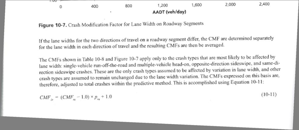
124 114

125 115

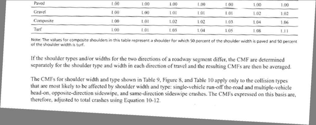
126 116

127 117

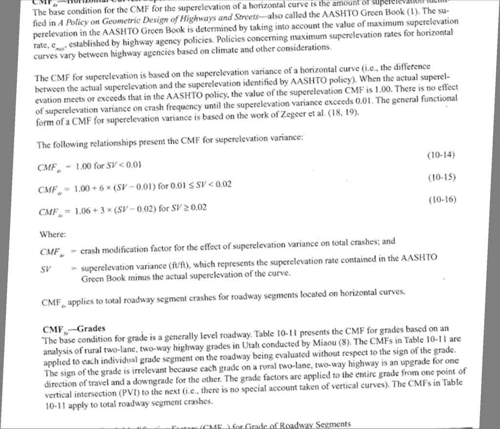
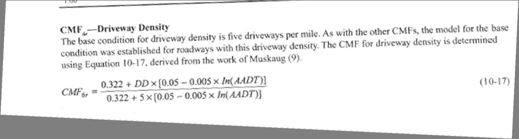
128 118